Table of Contents

• Announcements
• Laboratory Instructions
• Writing Reports
• Using the Simulation and Plotting Programs on Personal Machines
• Data Acquisition Programs
• Investigate the Ohmic Behavior of a Resistive Potential Divider Using a Waveform Acquisition Program

Announcements

• The first laboratory session is Tuesday 26 September at 9:00.
• The lab rooms will be open at 8:30 or earlier to 11:50 AM TuTh. However, the lab can be opened for students to work anytime by appointment.
• Always be in the lab at 9:00 as this will be the time for discussions of experimental instructions and data interpretation.

Laboratory Instructions

• Introduction to the electronics laboratory.
• Lab 1: Resistance.
• Lab 2: Capacitors and time-dependent RC circuits.
• Lab 3: Inductors and time-dependent RL circuits. Download the response spectrum package, the simulation package and the plotting package.
• Lab 4: RLC Circuits and Resonance.
  • Results for L = 330 μH (r is unknown) and C = 3.0 nF in parallel: input pulse and output in time domain; output in time domain; output in frequency domain.
  • Results for C = 3.0 nF in parallel with series combination of R = 51 Ω and L = 330 μH (r = unknown): input pulse and output in time domain; output in time domain; output in frequency domain.
  • Results in the frequency domain for the R+L||C circuit with L = 330 μH, C = 3.0 nF and R = 1.1kΩ: power spectrum; phase spectrum
  • Always save your data and simulations as csv files in a logical directory tree. To plot data and simulations on the same graph, use the latest version of the plot package. Open response_plot.py with Geany, and look at example 12 beginning at line 491 at the end of of the program. This plots one data file and one simulation file on the same graph. Notice that line 493 specifies the path to the data files relative to the plot directory: os.chdir('data/LC_parallel'). Modify this to point to your data files, which may require moving up one directory level: os.chdir('../data/LC_parallel'). This example has the legend switch set to True. If the legend covers part of the graph, just expand the size of the plot window. You can make you own run condition, beginning with if run == 13 :, but you must then change the number in line 261 to 13 as in run = 13.
• Lab 4i (no real lab report!) : Fourier transforms; using noise to measure A(ω), load vs cable impedance; transformers and mutual inductance; soldering. You will need the new Marina package for the FT experiments.
• Lab 5: Introduction to Operational Amplifiers. You will need one of these specification sheets: TL071 specifications; AD711. Also, read these notes: Introduction to Operational Amplifiers. To simulate the response of inverting and non-inverting opamp circuits, use the modularized simulate program package. Unzip this into a new directory in your programs directory tree. Remember to keep you recorded and simulated data in organized directories. As an example, unzip LC_LP.zip into you data directory tree and peruse the txt file, while describes the circuit and component values.
• Lab 6: Applications of Operational Amplifiers I, but only the "Summing Amplifier - Adding a DC Offset to an AC Signal" section.

Writing Reports

• Laboratory Report Suggestions (TA)

Using the Simulation and Plotting Programs on Personal Machines

• To use the simulation program and the plotting package referred to above, you must install Python and some Python packages. Since the simulation and plotting programs are not compatible with Python 3.x, use Python 2.7 in either the 32 or 64 bit forms for Linux, MacOS, XP or Windows 7 operating systems. Install these packages for your particular OS and Python version: numpy, scipy and matplotlib.

Data Acquisition Programs

• For acquiring data from oscilloscopes and controlling the output of the waveform generators, a Marina application is used. Marina is a Python package which enables any set of Python modules to work together and which provides a GUI for specific modules which involve user input and output. Log on as ph411, create the directory Desktop\ph411\python, download marina_ph411.zip and extract into Desktop\ph411\python . To execute the application, simply double-click on Desktop\ph411\python\marina_ph411\control.py.
• The Instrument page on the PH 415 Computer Interfacing site discusses the concepts of data acquisition for the AFG3021B (operations and programming manual) and TDS1012B (programming manual). The programs to be used in this course can be executed on any operating system with the following installed resources: Python, numpy or scipy, wxPython, matplotlib, pyvisa, a visa library and drivers for both instruments. On the laboratory XP machines, the visa.dll and niusbtmc.sys (driver) are part of the NI LabView installation. The preferred editor for the course is Geany, a syntactically-aware integrated development environment for all operating systems.

Investigate the Ohmic Behavior of a Resistive Potential Divider Using a Waveform Acquisition Program

• Set the function generator to provide a bipolar ramp at 100 Hz with V_pp = 1 V_pp into 1 MΩ. Set the oscilloscope to display your preference of black on white or white on black, both channels for 1 V_pp full scale, 2 cycles across the screen. On the acquire menu of the scope, press the (single) sample button. Another option would be to average over 64 waveform acquisitions, but the statistical analysis presented below is based on only single waveforms.
• Build a simple resistive divider with identical resistors and apply a bipolar ramp from the function generator. Make a thoughtful choice of resistors. How small can they be and not bias the measurements? How large can they be? Set the output impedance value on the function generator to the correct value. Connect this signal to channel 1 of the oscilloscope and the signal across the resistor to channel 2. Remember that the oscilloscope measures signals relative to earth ground! Use DC coupling. Set the trigger to external and the trigger level to 500 mV. Connect the TTL output from the FG to the trigger input of the scope.
• Set the oscilloscope to display two ramp cycles, with both waveforms scaled to use the entire dynamic range of the ADC (the entire vertical range of the display). Do not exceed the dynamic range, otherwise the ADC will saturate.
• Execute Desktop/ph411/python/marina_ph411/control.py, select the oscilloscope and acquire waveforms from both channels. Make a graph that has the information content you seek, scale it to you satisfaction and save as an eps and as a pdf. Save the data as a csv file, and try creating a spreadsheet.
• Do this also for 5 V_pp at 100 Hz and 5 V_pp at 250 kHz (the maximum ramp frequency).
• Use response_plot.py, response_plot_base.py and response_plot_files.py to makes plots of data stored in a csv file. The program is set to run example 7 using the data set xy.csv which is an xy data set acquired from the oscilloscope by scope_waveforms.py.
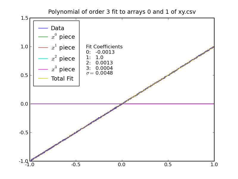
• Determine the validity of the assumed Ohmic behavior of the resistors under test. Fit a straight line indicative of Ohmic behavior to V₂(V₁). The program polyfit_fit.py on the Python page demonstrates how to use numpy to fit polynomials to data and to use the residuals as a measure of the certainty of the fit. To fit a polynomial to an approximately linear set of data in a csv file created by scope_waveforms.py, use fit_linear_data.py. The program can be executed directly if the data file is xy.csv. Otherwise, you will have to change the name in the program.
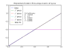
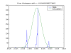
• Graphs of xy.csv: polynomial fit error histogram .
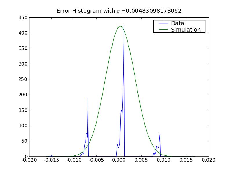
• Use the error histogram plotting capability of fit_linear_data.py to analyze the noise distribution of V₂(V₁). Note that the program also graphs the normal gaussian error function of the same σ. Explain the interesting experimental error distribution for the digitized data from the scope as in the analysis of xy.csv above. Consider that the oscilloscope performs 8 bit analog to digital conversion (ADC). The entire vertical range is then reduced to only 256 possibilities, from 0 to 255. As can be seen in scope_waveform.py, the waveform acquired from the oscilloscope consists of 16 bit (2 byte) integers, but the lower byte of each number is zero.
• V₂(V₁) should be linear unless there is non-Ohmic behavior on the part of one or both resistors or some other element in your experimental system. Does the polynomial fit to your data become more or less linear as the frequency ω and V_pp vary?