Malgorzata Peszynska

Flow & transport modeling

Flow and transport that we consider (here) is described by the traditional PDEs. Flow models are typically elliptic or parabolic, and transport models describe advection, diffusion, and reaction. Computational methods should be conservative, and higher accurate transport methods can help to prevent the smearing of the fronts. In complex geometries, the trick is to make sure that you have a conservative velocity field.

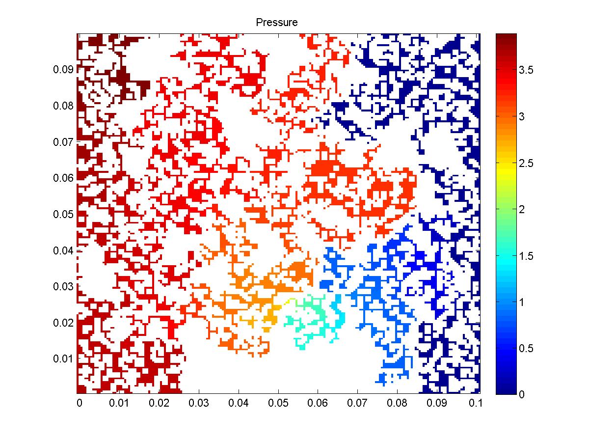
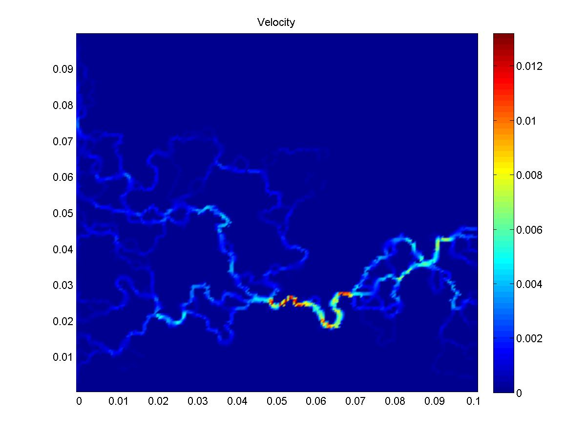
Pressure (left) and velocity field (middle) in complex geometry (actually, at the porescale, but this is not relevant here). Right: transport simulation in a similar geometry.
See also some flow and transport simulations at the porescale.

Multiscale modeling, analysis and simulation

One of the compelling examples of why we the multiple scales are important and challenging comes from the models and applications of flow and transport in porous materials. Our DOE multiscale grant involved modeling of preferential flow from meso- to macro-scale, and modeling from porescale to meso- scale. We first discuss the meso- to macro-scale problem. It is important when building large scale models (on the aquifer or hydrocarbon reservoir scale of kilometers) using coefficients measured in a laboratory from core samples, i.e., at the centimeter or meter scale.

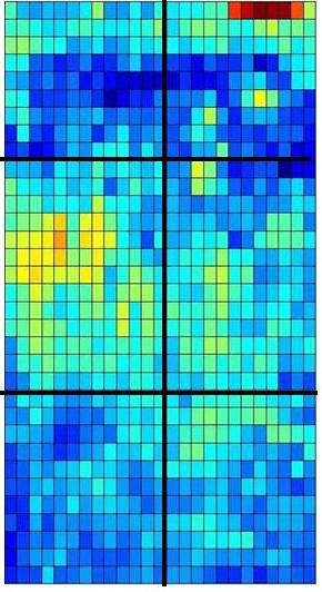
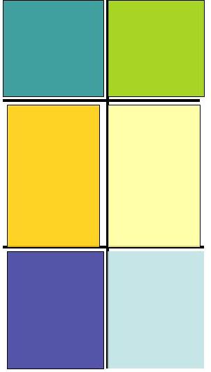
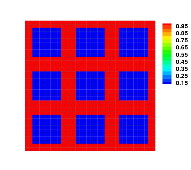
The "traditional" challenges in porous media were associated with heterogeneous and fractured (fissured) media. The difficulty is that the properties of the porous blocks in the matrix are very different from those of surrounding fractures, thus majority of flow and transport happens in the latter, while the storage is confined to the former. While one could, in principle, use very fine computational grids to resolve these fine details, this is not practical. Left pictures show the original and the upscaled permeability field. On the right we see an idealized "binary" medium: periodic fractured medium. Rather than attempt to solve problems at the fine scale, mathematicians have built upscaled models that work at the coarse scale, while incorporating the effects of lower scales.

Interesting things happen when you move to time-dependent and/or nonlinear models. The latter (with CG), e.g., for non-Darcy flow, can produce approximate upscaled models where you fit an effective model to some plausible algebraic form. In turn, the time-dependent case is quite interesting, especially if it comes from a coupled flow-transport model. With SY and RES we studied the case when the scales (contrast) are not well separated, and developed multiscale models with memory effects, represented by Volterra integrals with (weakly) singular kernels.

Now, even more interesting is the case when the model at lower (micro) scale is different than the one at higher (macro) scale. Such is the case of pore-2-core upscaling, when the lower scale flow models recognize the different physics (viscous flow-Navier-Stokes) from the upper scale (filtration laws such as Darcy's law). This case is part of our porescale modeling efforts and non-Darcy work. Things get even more interesting when the physics at different scales is completely different such as in the semiconductor project, where we used Density Fuinctional theory to calculate the properties of an interface handled by a jump condition in a continuum scale drift-diffusion (PDE) model. More broadly, this is why we started working on hybrid models which is what you need to put together model components of completely different types (such as centaur= body of a horse, and head of a human).

Non-Darcy flow and inertia effects

In the flow through porous medium, there is significant interaction of fluids with the surrounding rock grains, causing additional dissipation of energy (in addition to the internal friction). While at the porescale one still models the flow using Navier-Stokes or Stokes equations, the average flow satisfies non-Darcy's or Darcy's law; i.e. the momentum conservation equation. One interesting perspective is that the linear Darcy's law was discovered empirically with coefficients derived experimentally, and there is beautiful mathematical proof by homogenization (going back to the work of Tartar from 1980) that shows how Stokes equation can be averaged (in periodic geometries) to give Darcy's law.

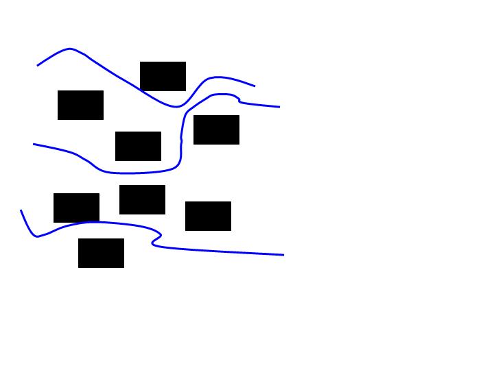
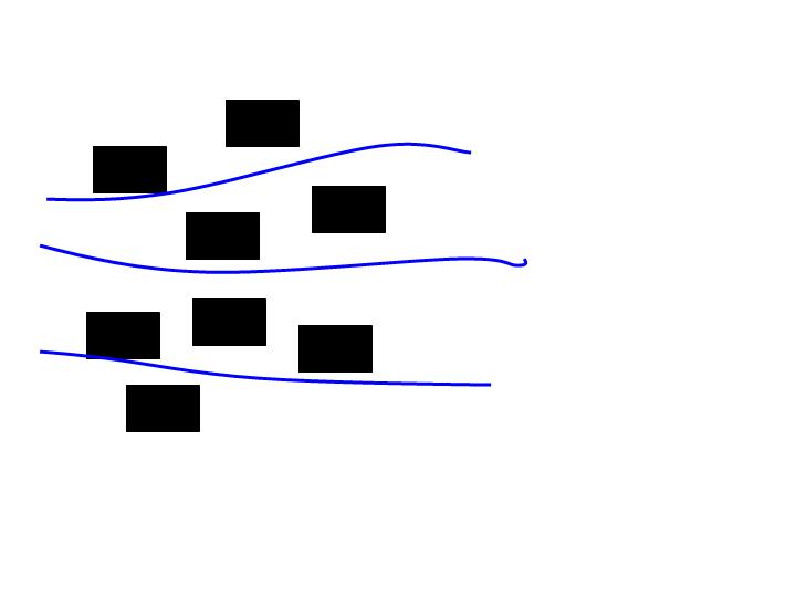
The cartoons illustrate the difference between viscous flow for high and low flow rates. At large flow rates, the flow paths tend to be more "straight", while at low rates they tend to be more "tortuous". For fluids in a river, ocean, or atmosphere, the PDE models of Navier-Stokes include the nonlinear advective term also called "inertia term". This term is dropped in the Stokes model which works well for low flow rates.

However, there is really not one universally agreed form of non-Darcy model, even though there have been attempts to generalize the 1d quadratic Forchheimer law to multiple dimensions and heterogeneous media. In our work we set out to use numerical averaging (homogenization or upscaling) to discover a general non-Darcy's law in our virtual laboratory. (See our porescale work and [PTrykozkoAugustson'2009, PTrykozkoKennedy'2010, and our other work joint with Dr A Trykozko '2010-; see also [GaribottiP'09 for upscaling non-Darcy flow].

Porescale modeling

Porescale modeling was once thought to be impossible, but is now very well developed. See Porescale Benchmark project, which evolved to Digital Rocks portal.

The first challenge in porescale modeling is to define WHY you want to do it. WHAT needs to be done is fairly obvious: you simulate the physical processes, and voila! Out come the simulation results (a lot of them). The WHY tells you what you can do with them, and the HOW is non-trivial.

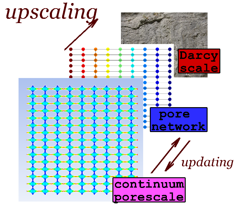
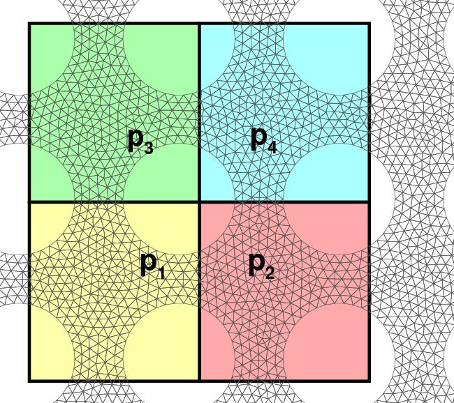
The image shows a heterogeneous porous rock (Darcy scale), which can be idealized as having periodic porescale geometry such as that shown in the background. At Darcy scale one solves a flow problem (e.g, an elliptic or parabolic PDE for the pressure). At pore-scale we solve the Stokes problem. One can next "upscale" from the Stokes scale to Darcy scale over a representative relementary volume using the setup such as shown on the right.

In particular, you need to consider methods of upscaling which will apply to nonlinear processes and non-periodic geometries, because otherwise you will always be stuck in an idealized-limbo about which almost all is known but from which it is difficult to move forward. You can use the linear periodic case for testing, but that's it.

In our first approaches, we approached high flow-rate (velocity) flow at porescale which is simulated with Navier-Stokes equations. When upscaling, this gives the collection of non-Darcy models, and, interestingly, there is no agreement to what they should be, especially if you want to consider anisotropy. We defined our own variant of upscaling via volume averaging, and (with KA and AT), were able to also identify appropriate anisotropic extensions of Forchheimer laws.

Then our appetite and curiosity grew. We wondered how much our findings depended on the "nice-ness" of the geometries. Hence, we started using real porescale data (sandstone, glass beads, tuff). Several colleagues shared with us their porescale micro-CT and Xray tomography data. The real fun started when the porescale was changing due to the presence of biofilm growing there, and eventually clogging some pathways.

The first movie (HS) was made using sandstone data from Brent Lindquist's group. The second movie (GB) was made using glass beads data from Dorthe Wildenschild's group. When we say "data" here, we mean we obtained the binary voxel data (e.g., 30M cells marked either as solids or as void). Then we applied fluid flow models. Visualization was done with Tecplot, and simulations with ANSYS Fluent. Watch out, there is music there to reflect our enthusiasm for the topic!

We continue efforts on modeling the flow at porescale when the geometry is changing, e.g, due to reactive transport, or phase transitions. For our first models, see [PTISW15] paper, and/or [TC] thesis, and/or [CKP18] paper.

The next example was made by Joe Umhoefer supported by NSF (DMS-1738014 and DMS-1522734), and it shows Eulerian and Lagrangian transport of particles at porescale, in a velociy field calculated by the software HybGe-Flow3D. See detailed description in "credits" to this movie, summarized below.

Eulerian and Lagrangian advective transport through a porous media shown on the left. On the right, we give the breakthrough curves for both, showing the solute output relative to the influx on the vertical axis, and time on the horizontal axis. Breakthrough curves for Eulerian transport in black, Lagrangian transport in red. Flow solution from HybGe-Flow3D (https://github.com/numsol/HybGe-Flow3D). Geometry Sourced from: [PTISW'16].

Methane hydrate: applications and math

To learn about methane (gas) hydrate, visit DOE-NETL hydrates page, USGS site , ORNL page .

I was fortunate to have been introduced to hydrate research by two colleagues from CEOAS, OSU, Marta Torres and Anne Trehu; see "Solving the world's real-life math problems" (December 2014 feature) on this collaboration. One of the challenges of hydrate modeling is that very few mathematical results were ever published on the topic prior to our work. Perfect for us! However, to understand the models first, we had to wade through the geochemistry and geophysics vocabulary, which is disparate from mathematical language. (They are similar but then they are not, like Spanish and Portuguese).

This video is a result of the first model we built. It is fully coupled, but we use the assumption of fixed and linearly varying pressure and temperature. Each graph is set-up in the way the geophysics community displays subsurface (horizontal axis is the variable, and the vertical axis shows the depth, which is quite natural when you get used to it). Details of this model are presented in the ICCS paper.

Since these initial models I worked with other collaborators and students on the hydrates. Our results include simulations, and analysis, with continued numerical analysis.

Mathematical framework we developed involves abstract evolution equations and complementarity constraints. These help to describe the so-called maximum solubility constraints which keep the amount of dissolved gas in the liquid phase from exceeding the bound imposed by thermodynamics. The hydrate (or free gas) form when the amount of gas exceeds the bound. Hydrate does not move, but free gas does, and there are still many mysteries involving the dynamics of this coupled system.

Our first approach was to study the entire system, see the movie from ICSS. Then we gradually disassembled the problem into smaller parts which we could analyze, as in the papers [GMPS'14, PSW'15]. Working from these most simple models towards more complex ones, we built in the coupling with the transport of salt, and the dependence of thermodynamics on the alt; see [PHTK'16] and [PMHT'16] which show how we solve the coupled system, and how our case study simulations compare with data from Ulleung Basin.

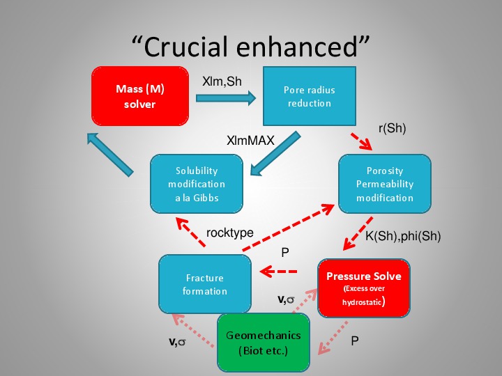
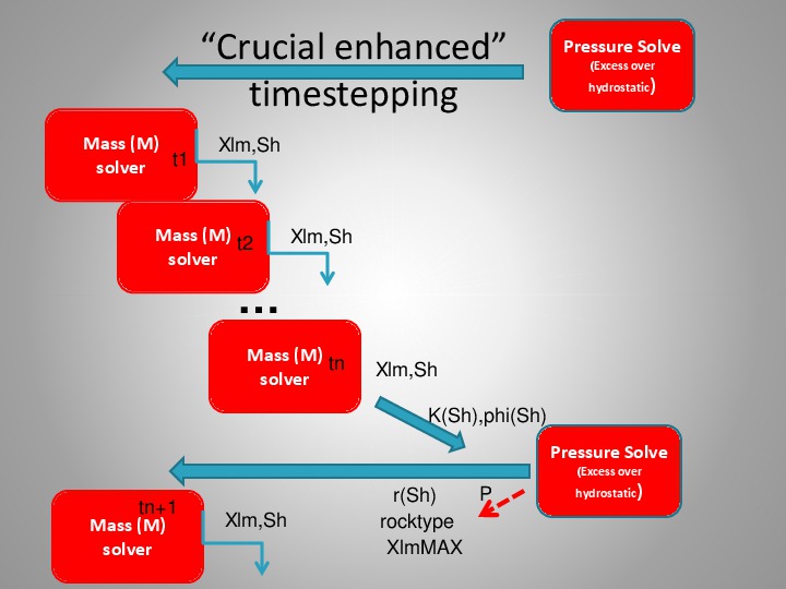
This video is my 2d simulation inspired by the 1d case study and model from the paper [DaigleDugan'2010]. The model accounts for the dependence of thermodynamic constraints on hydrate formation on the type of host rock in which it forms. We used our 2d "crucial enhanced" implementation of the reduced numerical model we described in [PHTK'16], enhanced by solving the pressure equation, and accounting for the formation of fractures based on the pressure threshold condition. The structure of coupled model is schematically depicted in the cartoons below. The geometry of the reservoir is inspired by that of Hydrate Ridge so that its top (in the middle) is higher than the sides. In the simulation, the red-to-yellow (hot colors) show the increase of methane hydrate saturation (Sh) caused by the migration of methane upwards from the bottom of the reservoir into the hydrate zone. The blue lines delineate rock types: initially, they differentiate between fine-grained (clay) and coarse-grained (silt) sediment. Over time the fractures form at the bottom which is shown as new rock type. The mild nonsymmetry is a visualization artifact, but the uneven migration and hydrate formation patterns are primarily due to the heterogeneity of the rock. The time scale is in [ky]! Gravity points downwards, and the top of the reservoir is the bottom of the ocean.

Our current work involves modeling hydrate formation at porescale to understand how it clogs the porescale. In particular, we are working on phase-field models. (More informaiton forthcoming). See also hybrid models.

Adsorption: classical and hybrid models

"Adsorption is a process in which the molecules of adsorbate form a film on the surface of adsorbent".

The videos explain the process, and how an equilibirum forms between the average amount adsorbed and the average amount present in the fluid. The second video shows the idea that in some geometries, a nonequilibrium can form due to nonequal access to the surface, and this would result in hysteresis. The third video (made by F.P.Medina) is a cartoon of the process of competitive adsorption involving multiple components.

One particularly important application of adsorption arises in the study of methane gas which occurs naturally in the subsurface reservoirs, e.g., in coalbeds (or shales). Enhanced coalbed methane recovery techniques attempt to recover methane by injecting other gases such as carbon dioxide.

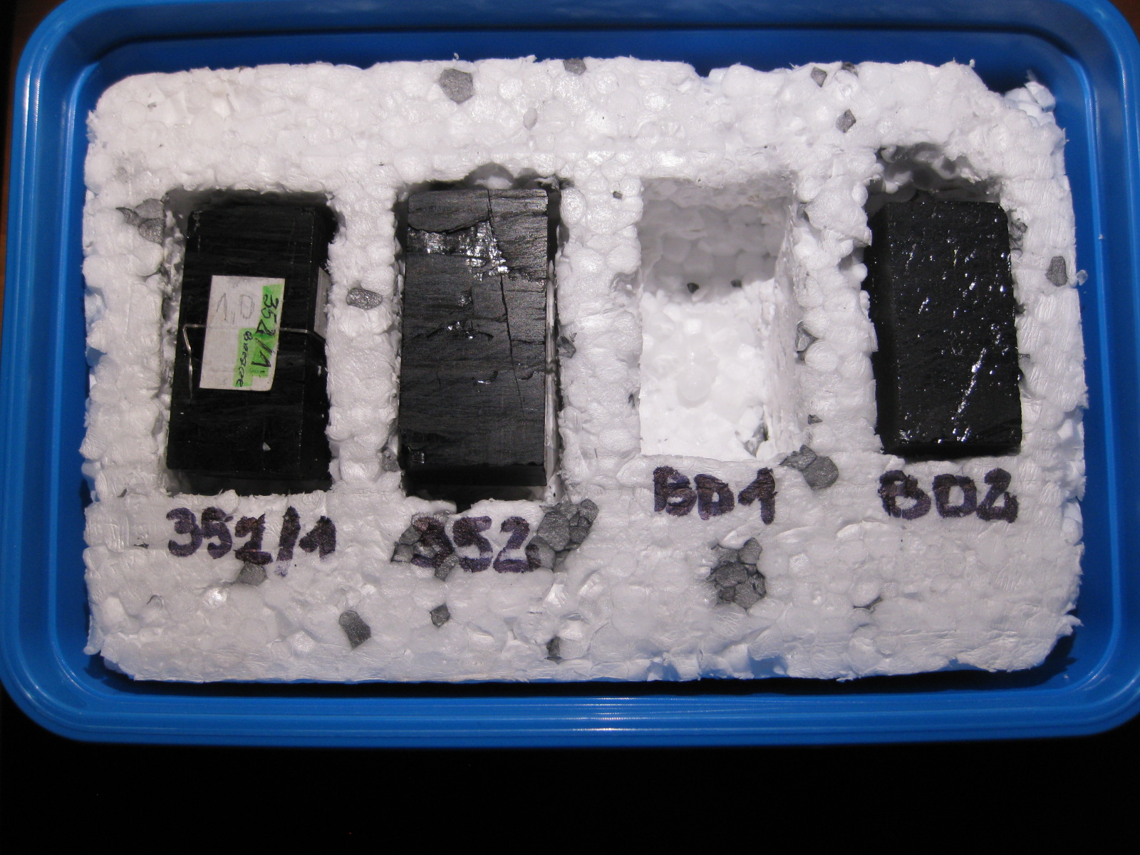
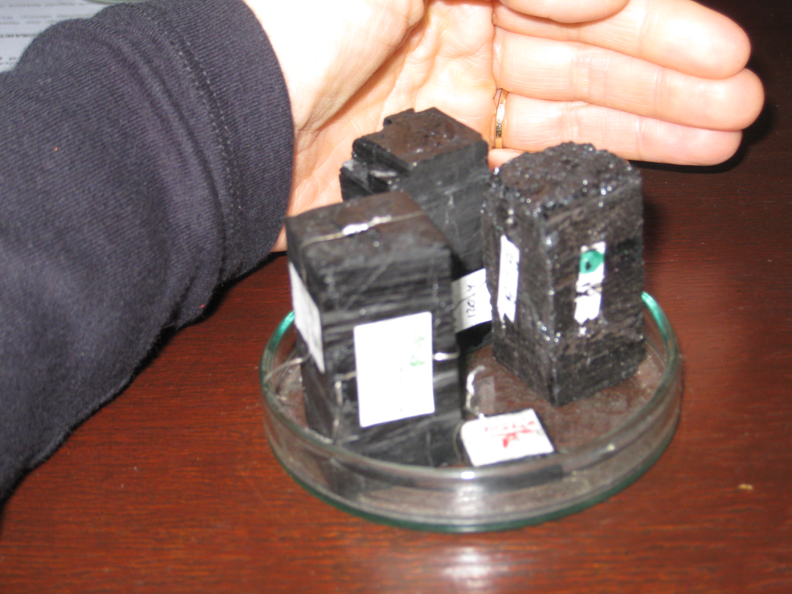
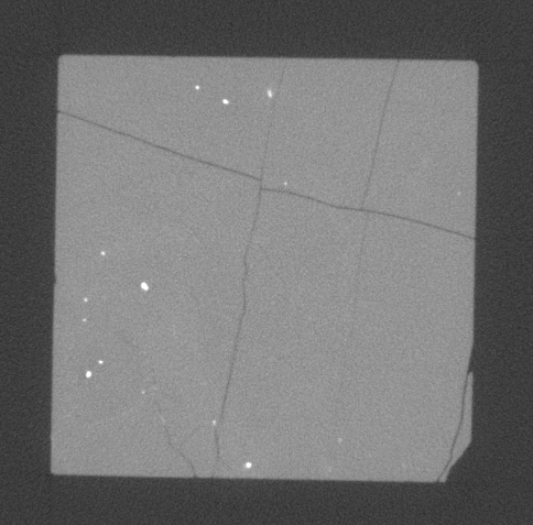
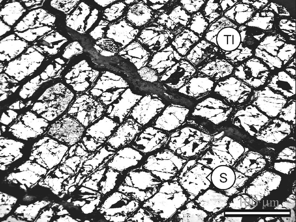
The images show samples of coal obtained from the lab at the University of Mining and Metallurgy in Cracow while I was on sabbatical as a Fulbright Fellow. The right image is a tomographic image of these samples which shows a "perfect" double-porosity structure of coal with fractures (cleats) crossing the matrix. The right-most image shows again the multiscale structure of coal. Since it involves (subscale) diffusion into the matrix, it causes memory effects.

Memory effects from non-equilibrium and subscale processes

Oh, the multiple scales. Sometimes the coefficients of a PDE model vary significantly in space. For example, such is the case of porous medium with fractures, where the permeability values in fractures may be 1000 larger than those in the remaining (bulk=matrix) part of the medium. At the same time, the fractures take up significantly less volume than the matrix. Another example is of composite engineered materials where, by design, one puts together materials with different properties (softness, hardiness) so as to achieve optimal overall performance. One can use homogenization (a rigorous and sophisticated version of averaging) to infer effective properties of such media at a higher scale.
Another example is that of viscous flow at the pore-scale described by the Stokes flow, which, after averaging, gives Darcy's law.
The memory effects arise when considering transient phenomena in multi-scale media such as flow and transport. The (slightly compressible) flow and/or diffusive transport in the two parts of the medium (of large and small permeability) occur at different time scales (fast and slow, respectively). However, the "slow" parts cannot be ignored since majority of the fluid resides there, and subsequently "feeds" the "fast" parts. In order not to have to adjust the spatial and time discretiation to both media at the same time, the idea is to use homogenization, and to include the "slow parts" as subgrid effects or "memory effects". Another example is the transport of gas in coal matrix with adsorption. In our work we studied the effects of such "memory effects" on the solutions to the PDEs, and proposed and analyzed efficient numerical schemes for these. In particular, see [P'2014, KleinP'2012], and work with S.-Y.Yi and R. Showalter'2008-2014]. Our earlier work includes that in [P'92-96]. The effect of memory effects on (nonlinear) conservation laws was studied, e.g, in [P'13].

Analysis of well-posedness and of properties of solutions

After one takes an introductory class on Partial Differential Equations (PDEs), everything is clear. Every PDE is of one of the canonical types, the boundary conditions are always homogeneous, and the data is always smmooth. Right? Thus, the classical solutions can be proved to exist and be unique. (So these PDEs are well-posed).
Well, it ain't exactly so in real-life. Most real-life PDE models studied today are nonlinear and coupled, and have nonsmooth coefficients. The well-posedness defines which data gives rises to a weaker notion of solutions, and how strict the assumptions on data need to be to get uniqueness, and how large the class of solutions needs to be to ensure existence of solutions. Of interest is also sensitivity of solutions to the data.
In our work we have contributed to the analysis of solutions to various real-life problems. The goal was to understand the structure of solutions so that they can be (later) approximated numerically, but many times the analysis itself was the point in itself. For example, there is no point in using a method (such as finite difference) which requires C⁴ smoothness, if your solutions are barely C⁰! Or, if you supply more boundary conditions than needed for well-posedness, no matter how fast your numerical method is, it will fail. As another example, in the process of studying the stability of solutions to the continuous model, one discovers whether stability can be expected from the numerical solutions. Finally, we also studied properties of solutions in the presence of interfaces, and the dependence of solutions on various coefficients.

Numerical analysis of flow and transport processes

Most models of real-life phenomena do not have closed form solutions. For example, in general, you cannot solve exactly polynomial equations of high order, or calculate integrals with some monstrously complex integrands, or solve high-order non-separable differential equations not amenable to some magic substitution.

However, one can approximate such solutions. Numerical Analysis is the study of algorithms for the approximations, and Scientific Computing is the field devoted to the most efficient computer implementation of the algorithms. Numerical Analysis assesses the error in approximation, and specifies under what assumptions the error converges to zero. It also suggests how to determine whether such an approximation is "good enough", for example by studying a-posteriori error estimates that help to determine whether to continue some iteration, or mesh refinement.

In our work, we have mostly considered numerical analysis for flow and transport problems. We derived a-priori and a-posteriori estimates for the approximations derived with Finite Element methods (Galerkin amd mixed methods), using domain decomposition and mortar couplings. We also considered stability in time and derived various conditions for (advective) transport dominated problems and problems with memory terms. We were also involved in HPC (High Performance Computing) projects (see [P et al 1998-2005]) in which methods proven stable and accurate for simpler problems were implemented, tested, and used for simulations of complex coupled multiphase multicomponent systems; see e.g. our hydrate projects.

Coupled nonlinear phenomena

Analysis and numerical analysis of scalar (differential) equations (when we solve for only one unknown) is fairly well developed. Coupled phenomena such as flow & geomechanics, or flow & transport, require that we solve for several unknowns which appear in several equations. The first common difficulty is that the coupled system has a structure that does not have a familiar structure, say of elliptic or parabolic type. Moreover, the coefficients of the coupled system frequently depend on other uknowns, can degenerate (go to 0) or get singular (blow up), thereby changing the type or the expected qualitative properties of the solutions. A particular class of coupled systems is in the modeling of multiphase multicomponent flow and transport such as in groundwater contamination scenarios or oil and gas recovery reservoir simulation. Another important class is of (very nonlinear) coupled system modeling interface evolution in phase transition models such as the Cahn-Allen and Cahn-Hilliard equations.

Important keywords: solvers, multiphysics, multinumerics.

Hysteresis and monotone operators

Simply put, hysteresis occurs when the output depends on whether the input is increasing or decreasing. This means that there are multiple outputs corresponding to each input, i.e., a relationship with hysteresis is not a function.

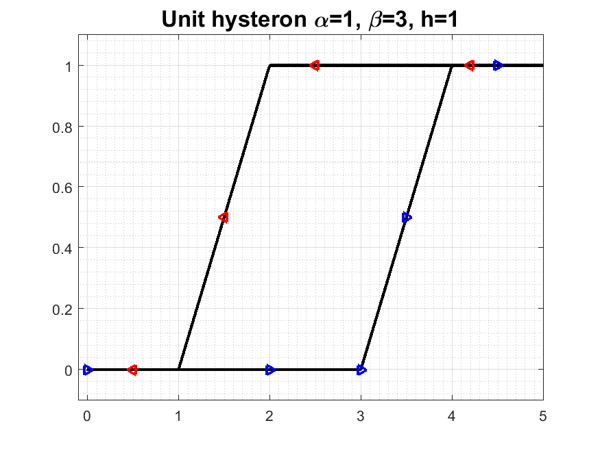
The graphs show a hysteresis operator with a piecewise linear output, and the corresponding movies show the evolution. There are multiple outputs w corresponding to a particular input, e.g, u=3. The value w depends on whether the input u(t) is increasing in time t or decreasing (see arrows and the movie).
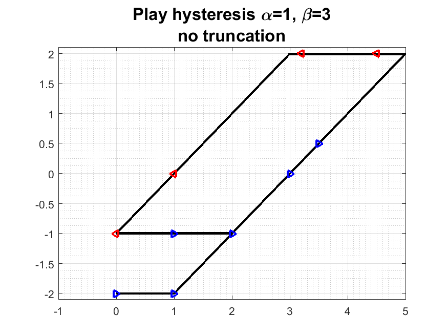
The first movie/graph show the simple "play hysteresis". In each frame of the movie, on the right, you see the input u(t), together with the corresponding w(t) which is "dragged" by u(t). On the left you see the phase portait of the graph in (u,w) plane. A linear combination of "play hysterons" was the model we analyzed in [PS97].
The second movie/graph show what we call the "unit hysteron", which takes the same input as the play example, but the output is truncated.

Hysteresis is an important phenomenon, common in electromagnetics, and quite common in modeling flow and transport in porous media such as capillary pressure drainage and imbibition and/or adsorption hysteresis. Our examples here come from, and are useful for, the latter class of applications.
Models of hysteresis are challenging, because they require extension of a notion of a function to a (multivalued) operator or graph. This makes the analysis of, and approximation to the solutions to models which involve hysteresis, exciting enough!
A very useful but also very complex construction of hysteresis operators follows the notion of Preisach hysteresis. We have developed another class of models based on a simple construction of an ordinary differential equation under a constraint. In [PS97] we analyzed the solutions to a transport model with a particular convex-concave hysteresis operator; the crucial observation was that thanks to the convex-concave character of the graph, the solution was more rgular than in the usual C^0(L^1)setting; in particular, it was continuous.

Recently (see forthcomng paper [PS18]), we have extended the hysteresis models to include realistic graphs such as the adsorption/desorption hysteresis graph. This is achieved with the help of a truncation functional which helps to isolate individual portions of the graph. However, due to the additional nonlinearity in the construction, the solutions can only be analyzed in the C^0(L^1) setting on a product space. The added benefit is the ability to calibrate any reasonable experimental graph with a simple adaptive procedure.

Random or unknown data, uncertainty, and stochastic simulations

Forthcoming ...

Hybrid modeling

Broad description forthcoming ...

The simulations show how you can use a version of Metropolis algorithm to find an equilibrium configuration of fluid (red) in the presence of porous medium (black squares). here the preference to aggregate and to adsorb are controled by the proportion of parameters wff and wmf.