Chapter 5: Black Holes
- §1. Extending Schwarzschild
- §2. Kruskal Geometry
- §3. Penrose Diagrams
- §4. Charged Black Holes
- §5. Rotating Black Holes
Penrose Diagrams
A Penrose diagram is a spacetime diagram in which points at infinity are included. This is accomplished by rescaling the metric, that is, replacing $ds^2$ by $\Omega^2\,ds^2$, where the conformal factor $\Omega$ typically behaves like \begin{equation} \Omega \sim \frac{1}{r} \end{equation} Points with $\Omega=0$ therefore correspond to points “at infinity”; more formally, this construction adds a conformal boundary to the original spacetime. Since the metric has merely been rescaled by the conformal transformation, lightlike directions are preserved, and it is customary to continue to draw such directions at $45^\circ$. Penrose diagrams are usually drawn in two dimensions, with angular degrees of freedom suppressed; a “point” in a Penrose diagram typically represents a two-sphere. For this construction to work, the spacetime must be asymptotically flat, which roughly speaking means that it must look like Minkowski space “far away”. All of the spacetimes we have considered so far are asymptotically flat.
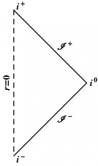
The Penrose diagram for Minkowski space is shown in Figure 1. Angular degrees of freedom are not shown; this is the $rt$-plane. The dashed vertical line represents the coordinate singularity at $r=0$; you can imagine the diagram being rotated about this axis, although each point with $r\ne0$ corresponds to a sphere, not a circle. In Minkowski space, there are five different ways of getting infinitely far from the origin. Three are fairly obvious: far away in distance (spatial infinity, denoted $i^0$), and far away in time, either to the future or past (two timelike infinities, denoted $i^\pm$). Each of these infinities corresponds to a single point in the Penrose diagram, which can be thought of as 1-point compactifications, analogous to the process of mapping a plane to a sphere using stereographic projection, thus adding a single “point at infinity”.
However, in Lorentzian signature, light behaves differently, and there are also two further pieces to the conformal boundary, representing the final destination of outgoing radiation and the source of incoming radiation. These boundaries are referred to as future and past null infinity, denoted $\II^\pm$, and called “Scri”, for “script I”. Penrose diagrams, conformal boundaries, and asymptotic flatness were all developed as tools for understanding radiation in general relativity, both electromagnetic and gravitational. Ironically, none of the early examples of asymptotically flat spacetimes, including those considered here, in fact contained any such radiation; it was only later that nontrivial asymptotically flat spacetimes were shown to exist.
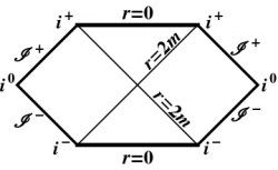
The Penrose diagram for the maximally extended Schwarzschild spacetime, the Kruskal geometry, is shown in Figure 2. The thin lines represent the horizons at $r=2m$, the heavy lines represent the singularities at $r=0$, and the remaining lines represent null infinity, with $r=\infty$. As discussed in the previous section, the horizons divide the Kruskal geometry into four regions. The original Schwarzschild region with $r>2m$ is the righthand asymptotic region (“us”). The upper quadrant with $r<2m$ represents the black hole region, and the lower quadrant is a time-reversed copy, corresponding to a white hole. There is also a second asymptotic region on the left (“them”), which cannot communicate with the righthand region.
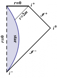
The Kruskal geometry does not correspond to any objects observed in nature; white holes do not appear to exist. A more realistic model of a black hole is one created by a collapsing star, as shown in Figure 3. The curved line represents the surface of the star; everything to the left of this line is inside the star, and the dashed vertical line represents $r=0$. As the star collapses, it eventually shrinks inside its Schwarzschild radius $r=2m$, after which a black hole forms. In this model, there is no white hole region, nor is there a second asymptotic region.
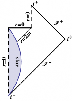
Hawking has proposed that quantum mechanical processes will cause a black hole to evaporate by emitting radiation. This process is known as Hawking radiation, and can be thought of informally as a spontaneous fluctuation in the quantum vacuum, creating a pair of particles “at” the horizon, with a positive-energy particle escaping to infinity, and a negative-energy particle falling into the black hole, thus decreasing its mass. A Penrose diagram for this model is shown in Figure 4. Nobody knows what happens at the point in this diagram where the black hole disappears (at the corner where $r=0$ and $r=2m$ intersect); the necessary theory of quantum gravity does not yet exist.