ANNOUNCEMENTS
MTH 437/537 — Spring 2024
- 6/15/24
-
The exams have been graded, and course grades assigned, although you may
not be able to see them until tomorrow.
-
If you have any questions about how your final was graded or about
your course grade, please contact me.
-
Answers to questions not asking you to show something are below.
-
-
(b) $\frac{3m\pm\sqrt{9m^2-8q^2}}{2}$
-
(a) $2\pi A$, $2B$
-
$f(\rho)=\frac{m-\rho}{m+\rho}$,
$h(\rho)=\frac{(m+\rho)^2}{2\rho^2}$
(constants may be different)
-
IF your grade were determined only by your final exam, it would be
(out of 70; extra credit included):
-
- $\ge63$: A
- 60–62: A−
- 55–59: B+
- 47–54: B
- 36–46: C
- 31–35: C−
- 6/11/24
-
Today's office hours via Zoom are confirmed for 1:30–3:30 PM.
-
Other times may be possible, and of course feel free to ask me
questions via email.
- 6/10/24
-
My office hours today via Zoom are confirmed for 1:30–3:30 PM.
-
As noted below, the Zoom link is available as a Canvas announcement.
Please be patient if you are not admitted immediately.
-
Kieran Edward Dray was born Saturday evening.
-
Mother and baby (and the rest of us) are doing fine.
- 6/9/24
-
In problem 2, you may assume that the cosmological constant vanishes, that
is, that $\Lambda=0$.
-
Please also remember that there are known errors in some of the results in
the appendix of the textbook; see the
errata page.
- 6/6/24
-
The Sage notebook I demonstrated in class for the Kerr metric can
be found here.
-
This version uses an orthonormal frame but Sage takes much longer to
compute the Riemann tensor using this method (quite possibly due to
inefficient programming on my part). A version that uses the definition
of the Kerr geometry that is built in to Sage using a coordinate basis
can be found here,
-
I will hold office hours via Zoom on Monday (6/10) and Tuesday (6/11) at
times to be announced, but most likely 1:30–3:30 PM.
-
The Zoom link has been posted as a Canvas announcement (and is the same
as the link we used last term).
-
Other times are possible; ask! I will also respond as quickly as possible
to questions sent via email.
- 6/5/24
-
The take-home final will be distributed online on Friday morning,
6/7/24, at 8 AM.
It will be due on Gradescope 48 hours from when you download it, but no
later than midnight on Wednesday, 6/12/24.
-
-
The final covers Chapters 1–9 in the text.
-
It is fair to assume that all exam questions can be answered based on
mastery of the material we have covered in class.
-
I will be available during the exam. Some times will be scheduled and
posted here, but you can also contact me via email to request an
appointment.
-
You may use any non-human resources you wish, except
exam or homework solutions from previous years.
(For the purposes of this exam, ChatGPT or similar AI engines count as
human.)
-
You may not discuss the exam with anyone other than me during
the exam period, even after you have turned it in.
-
With apologies, it appears that I never posted the curve on the midterm.
IF your grade were determined only by your adjusted midterm score
(rounded to the nearest integer if necessary), it would be:
-
- $\ge24$: A
- 22–23: AB;
- 19–21: B
- 17–18: BC
- 15–16: C
- 13–14: C–
- $\lt13$: F
- 6/4/24
-
With apologies for the last-minute confirmation, class will meet as usual
today.
-
(I was excused from jury duty.)
- 6/1/24
-
When using online resources to determine the Einstein tensor, be sure you
know whether the calculation is being done in an orthonormal basis, or,
more likely, in a coordinate basis. Although the
computational methods are quite different in these two cases, it
is straightforward to compare the answers obtained:
-
Tensor components always transform with the appropriate change of basis
matrix; that's what makes them tensors.
-
This transformation is especially simple in orthogonal coordinates, where
$\sigma^i = h^i dx^i$ (no sum) for some functions $h^i$.
-
For example, the statement that the Einstein tensor for the
Robertson–Walker geometry has a component
$G_{rr} = -\left( \frac{2a\ddot{a}+\dot{a}^2+k}{1-kr^2} \right)$
in a coordinate basis really means that the (symmetric, rank-2,
covariant) tensor $G$ has the form
$$G = ... - \left( \frac{2a\ddot{a}+\dot{a}^2+k}{1-kr^2} \right)
dr\otimes dr + ...$$
(where we often omit "$\otimes$", as when writing the line element).
Since we know that $\sigma^r=\frac{a}{\sqrt{1-kr^2}}\,dr$, we can rewrite
this expression as
$$G = ... - \left( \frac{2a\ddot{a}+\dot{a}^2+k}{a^2} \right)
\sigma^r\otimes\sigma^r + ...$$
from which it is clear that
$G_{rr} = -\left( \frac{2a\ddot{a}+\dot{a}^2+k}{a^2} \right)$
in an orthonormal basis (which some authors write as
$G_{\hat{r}\hat{r}}$).
-
Both of these expressions can be written as
$G_{rr}=-\left( \frac{2a\ddot{a}+\dot{a}^2+k}{a^2} \right) g_{rr}$, so
long as $g_{rr}$ is expressed in the appropriate basis.
-
Since the components of $d\rr$ are the identity matrix in any
basis, that is, since $g^i{}_j=\delta^i{}_j$, tensor components are
easiest to compare when they have this "one up, one down" index structure,
that is, as vector-valued 1-forms.
-
Sage code that computes the curvature for the Robertson–Walker
geometry can be found here.
- 5/30/24
-
A discussion of Birkhoff's Theorem can be found in the
Appendix.
-
The Sage code I demonstrated in class today can be found
here.
- 5/28/24
-
As announced in class today, you may use computer algebra to perform the
computations needed on HW #7.
-
As usual, you must document doing so, by attaching a printout of your
session and explaining at least briefly what the computations mean.
-
As also announced in class today, the final exam will be a take-home
exam. My current plan is outlined below; please let me know as soon as
possible if you have any concerns about these arrangements.
-
-
Ground rules will be provided, but the short version is that you may
use most software and/or online resources (with proper documentation),
but may not discuss the exam with anyone but me.
-
You may NOT use solutions from prior versions of this class, however
obtained.
You may NOT use automated resources such as ChatGPT.
-
The exam will be released via Gradescope on Friday, June 7, and
due on Wednesday, June 12; exact times to be announced.
-
HOWEVER, you will only have 48 hours from the time you download the
exam to complete the exam and upload it to Gradescope. Plan
accordingly!
-
I will hold Zoom office hours during the exam; use them! I may also
be available at other times.
- 5/25/24
-
All indices can be raised and lowered with the metric.
-
For example, since $\TT=T^i{}_j\sigma^j\ee_i$, we have
$\ee_k\cdot\TT = T^i{}_j\sigma^j\ee_k\cdot\ee_i
= g_{ki}T^i{}_j\sigma^j = T_{kj}\sigma^j$
and similarly for $\RR$ and $\GG$.
- 5/24/24
-
Several examples have been posted using Sage, including:
-
-
Further details about geodesic deviation can be found in §7 and
§A.2 of the text, both of which can also be found
here.
-
There are minor typos in the Schwarzschild curvature 2-forms as given in
§A.3 of the text:
-
The coordinate expressions in the middle of Equations (A.52) and
(A.53) are each missing a factor of 1/2.
Also, the initial minus sign should be removed from Equation (A.61).
-
However, the final expressions in terms of an orthonormal frame are
correct.
-
The
wiki version has been corrected, and a full list of errata
can be found
here.)
- 5/22/24
-
Here are my expectations for HW #6, due tomorrow:
-
-
Anything you calculate by hand needs to be explained with enough
detail that the logic is clear.
-
Anything you calculate by machine needs to be documented by attaching
a printout of your session, along with a (separate) brief explanation.
-
This explanation should make clear what software you used, what
conventions you used, and what the inputs and outputs were.
-
Giving the inputs and outputs does NOT require you to write
mathematical expressions; a brief description in words is sufficient.
-
No interpretation of the Ricci curvature is expected.
-
I do not expect you to typeset long and messy formulas.
- 5/21/24
-
A corrected version of the SageMath computation of the curvature of
Schwarzschild geometry in rain coordinates shown in class today can be
found here.
-
This version also substitutes $r=r(R,T)$ back in at the end. Compare the
result with the computation in Schwarzschild coordinates also shown in
class today, which can be found
here.
- 5/16/24
-
There are several computer algebra packages available for computing
curvature components:
-
-
A relatively recent option is to use the
SageMath cloud server. For
example, the calculation of the curvature 2-forms for the
Schwarzschild geometry shown in class today can be found
here.
-
One of the best has been the Maple package
GRTensor,
although I have not used the latest version, GRTensorIII.
-
Rough instructions on using the newer DifferentialGeometry
package, available in recent versions of Maple to compute curvature
tensors can be found here.
-
Another option is the Mathematica code written to accompany Hartle's
textbook, which is available
online.
-
Finally, there is a fast but clunky LISP program
called SHEEP (aka CLASSI), which is available on
the ONID shell server, shell.onid.oregonstate.edu.
(See below for instructions.)
-
Printouts of (old!) sample computer algebra sessions are available for
GRTensor
and CLASSI.
-
Older versions of my instructions, that also include coordinate-based
computations, are available for
Maple and Mathematica packages,
and for SHEEP/CLASSI.
-
You may use software to compute curvature on the homework!
See me if you would like help getting started.
-
You must however document doing so, and it's up to you to ensure that you
are working in an appropriate basis.
- 5/15/24
-
Answers to the midterm questions are below. Solutions will be discussed
briefly tomorrow in class, and can also be seen in my office.
-
-
(a) $24\pi m$
(b) $12\sqrt3\pi m$
-
(a) No
(b) $1/\rho$
(c) $\boldsymbol{\hat\alpha}$
(d) $-1$
(e) $1/\rho^2$
-
(a) $\rho\,\boldsymbol{\hat\alpha}$
(b) $\rho^2\dot\alpha$
(c) Many answers possible, including $\rho=e^{\pm\alpha}$
-
(a) $r=m\pm\sqrt{m^2-q^2}$
(b) $-\sqrt{\frac{2m}{r}-\frac{q^2}{r^2}}$
(c) No
- 5/14/24
-
Further information about charged and rotating black holes and their
Penrose diagrams can be found in the undergraduate
textbook by d'Inverno, which is available in the OSU library.
-
A more advanced treatment can be found in the book The Large Scale
Structure of Space-Time by Hawking & Ellis, which is also
available in the OSU library.
- 5/12/24
-
During Thursday's review, I remarked that the Gaussian curvature needed
for HW #5 can be computed as usual either extrinsically (use your
embedding in $\EE^3$) or intrinsically (use the structure equations).
As noted by one student, there is a third method: Since the surface of
revolution is isometric to the ($r,\phi$)-plane of the Schwarzschild
geometry, you can use the Schwarzschild curvature 2-forms given in the
text!
-
Yes, these curvature 2-forms, given in Appendix A.3 of DFGGR, are for the
full, 4-dimensional Schwarzschild geometry. But a major advantage of
working with differential forms is that you can always "use what you know"
in order to restrict given results to subspaces. Here, it is enough to
note $\Omega^\phi{}_r$ from (A.55).
(Be careful with the signs, although it is not actually necessary to work
out $\Omega^r{}_\phi$ using (A.57), since the Gaussian curvature is
independent of orientation.)
- 5/11/24
-
My review notes can be found here.
-
A list of topics suggested by previous students can be found
here.
-
I will hold extra office hours on Monday, 5/13.
-
I should be in my office from 11 AM–2 PM, although I will take a
lunch break at some point.
- 5/9/24
-
As announced in class today, the midterm will not contain any
questions about curvature.
-
Questions involving geodesics could involve determining the
connection, but can likely be answered using the symmetry techniques
discussed in class and reviewed today.
- 5/8/24
-
As mentioned in class last week, there are 10 independent Killing vectors
in 4-dimensional Minkowsk space, namely 4 translations: $\xhat$,
$\yhat$, $\zhat$, $\Hat{t}$; 3 rotations:
$r\,\phat=x\,\yhat-y\,\xhat$, $y\,\zhat-z\,\yhat$, $z\,\xhat-x\,\zhat$;
and 3 boosts: $x\,\Hat{t}+t\,\xhat$, $y\,\Hat{t}+t\,\yhat$,
$z\,\Hat{t}+t\,\zhat$.
-
Each of these Killing vectors can be realized as coordinate symmetries
of the line element in appropriate coordinates, e.g. by switching to
round (spherical or cylindrical) or Rindler-like coordinates.
-
It is straightforward to show that each of the above vectors satisfies
Killing's equation, namely $d\XX\cdot d\rr=0$. Less obvious (but not
difficult to show) is that these are the only independent solutions
of that equation.
-
The collection of all Killing vectors forms a Lie algebra under
the operation of commutation, where vector fields act on each other by
differentiation. Lie algebras are infinitesimal versions of Lie
groups, representing continuous symmetries. For (some) further
information, see
Chapter 10 of our
octonions book.
5/7/24
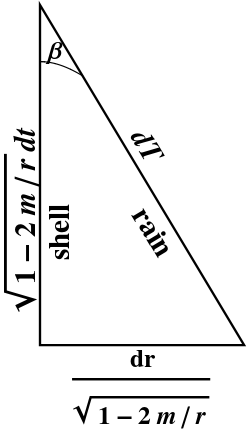 Figure 3.9 on page 38 (also available as Figure 8 in
this section),
showing the relationship between shell coordinates and rain coordinates, is
correct but misleading.
This figure shows the relationships between certain
differential forms, using the geometric description of
§13.8,
but without displaying the stacks. However, it is not easy in such
diagrams to read off the magnitudes of the differential forms, which do
not correspond directly to the lengths of the sides.
A more traditional figure, using the language of infinitesimal
displacement, is shown at the right.
Spacetime diagrams implicitly show relationships between vectors.
For example, the figure at the right shows that
$$d\rr = \sqrt{1-\frac{2m}{r}}\,dt\,\Hat{t}
+ \frac{dr\,\Hat{r}}{\sqrt{1-\frac{2m}{r}}}
= dT\,\Hat{T}$$
if $dR=0$, that is, for a freely-falling object. Figure 3.9 shows
instead a relationship between 1-forms, namely that
$$1\,\sigma^T = \frac{\sigma^t}{\sqrt{1-\frac{2m}{r}}}
+ \frac{\sqrt{\frac{2m}{r}}\,\sigma^r}{\sqrt{1-\frac{2m}{r}}}$$
which is always true.
(The explicit inclusion of orthonormal basis 1-forms restores the proper
scaling to the triangle.)
Figure 3.9 on page 38 (also available as Figure 8 in
this section),
showing the relationship between shell coordinates and rain coordinates, is
correct but misleading.
This figure shows the relationships between certain
differential forms, using the geometric description of
§13.8,
but without displaying the stacks. However, it is not easy in such
diagrams to read off the magnitudes of the differential forms, which do
not correspond directly to the lengths of the sides.
A more traditional figure, using the language of infinitesimal
displacement, is shown at the right.
Spacetime diagrams implicitly show relationships between vectors.
For example, the figure at the right shows that
$$d\rr = \sqrt{1-\frac{2m}{r}}\,dt\,\Hat{t}
+ \frac{dr\,\Hat{r}}{\sqrt{1-\frac{2m}{r}}}
= dT\,\Hat{T}$$
if $dR=0$, that is, for a freely-falling object. Figure 3.9 shows
instead a relationship between 1-forms, namely that
$$1\,\sigma^T = \frac{\sigma^t}{\sqrt{1-\frac{2m}{r}}}
+ \frac{\sqrt{\frac{2m}{r}}\,\sigma^r}{\sqrt{1-\frac{2m}{r}}}$$
which is always true.
(The explicit inclusion of orthonormal basis 1-forms restores the proper
scaling to the triangle.)
- 5/6/24
-
With apologies, I neglected to update the course website over the weekend.
-
There is an assignment this week, which is
hopefully reasonably straightforward.
-
Please let me know if this short timeline is an issue for you.
-
The formula sheet for the midterm has
been posted.
- 5/2/24
-
There are two competing usages of "rain coordinates", due to the confusion
between the two radial coordinates.
-
-
The Painlevé–Gullstrand coordinate system uses
coordinates $(T,r,\theta,\phi)$.
-
The rain frame uses basis 1-forms
$\sigma^T=dT= dt + \frac{\sqrt{\frac{2m}{r}}}{1-\frac{2m}{r}} \>dr$,
$\sigma^R = \sqrt{\frac{2m}{r}} \>dR
= \frac{dr}{1-\frac{2m}{r}} + \sqrt{\frac{2m}{r}} \>dt$.
-
(The basis 1-forms $\sigma^T=dT$, $\sigma^R$ in rain coordinates are
defined in
§3.9,
but the rain cooordinate $R$ is not defined until
§A.4).
-
So "rain coordinates" should really refer to $(T,R,\theta,\phi)$, but is
usually used as a synonym for Painlevé–Gullstrand coordinates.
-
Only the latterformer alternative corresponds
to an orthogonal coordinate system, with line element
$$ds^2
= -dT^2 + \frac{2m}{r}\,dR^2 + r^2 (d\theta^2+\sin^2\theta\,d\phi^2)$$
where $r$ is now an implicit function of $T$ and $R$.
-
Another way to see that surfaces with $\{T=\hbox{const}\}$ are flat is to
note that $\sigma^R-\sqrt{\frac{2m}{r}}\,\sigma^T=dr$, so that
$\sigma^R=dr$ if $dT=0$.
However, as pointed out in class, the $T$ and $R$ directions are
orthogonal, but not the $T$ and $r$ directions.
-
Thus, the operator "$\frac{\partial}{\partial T}$" is ambiguous! Holding
$R$ fixed, the resulting "$T$ direction" is not a symmetry, since the line
element above depends on $T$ (through $r$). Holding $r$ fixed instead
does lead to a symmetry; the Painlevé–Gullstrand line element
has no $T$ dependence. However, the resulting "$T$ direction" is
orthogonal to $r$, not $R$ — and is hence the same as the
Schwarzschild $t$ direction, which we already know is a symmetry.
- 4/30/24
-
The midterm will be Tuesday, 5/14/24 (Week 7).
-
The main topics to be covered on the midterm are:
-
-
Line elements;
-
Spacetime diagrams;
-
Geodesics and their properties;
-
Schwarzschild geometry.
-
Further information:
-
-
The exam is closed book;
-
There will be a review during Thursday's class on 5/9/24.
Come prepared to ask questions!
-
A formula sheet will be provided, and will be discussed at the review.
(A draft copy will be posted here
prior to the review.)
- 4/23/24
-
The due date for the assignment due today at 4 PM (HW #3) has been
extended until 4 PM on Thursday, 4/25/24.
-
You may resubmit your assignment without penalty until then.
(Assignments will not be accepted after the extended due date.)
- 4/21/24
-
When working on this week's assignment (HW #3), the discussion of circular
orbits in
§3.6 of DFGGR may be helpful.
-
As discussed both in class and in this section, we argued that $\dot r=0$
implies that $V'=0$.
- 4/19/24
-
The figures shown at the end of class yesterday can be found in
§3.5
of the text.
-
Here are some hints for this week's assignment:
-
-
For timelike trajectories, the 4-velocity $\vv=\frac{d\rr}{d\tau}$
always satisfies $\vv\cdot\vv=-1$; its magnitude is not the
speed.
-
Speed is distance over time. How far did you go? How long did it
take?
-
All measurements use the metric (line element).
-
The far-away observers introduced in the second problem
are not aware they live in a curved spacetime, so they (incorrectly)
use the Minkowski line element.
Note Added:
They use the Minkowksi line element when calculating, but
they use the same data as other observers.
- 4/18/24
-
Further information about the difference between the geometric radius and
the physical radius can be found in my
recent paper
on embedding diagrams, which was published
here.
-
A construction of the Schwarzschild embedding diagram is included, which
should be accessible to students in this class.
- 4/15/24
-
From the tagline of today's xkcd comic
strip:
-
The standard North American NAD83 coordinate system is misaligned from the
actual Earth, off-center by about 7 feet.
- 4/11/24
-
We didn't quite get to the derivation of the geodesic equation on the
sphere...
-
The answer can be found in
§19.3.
-
Solutions of the geodesic equation in polar and spherical coordinates can
be found in
§19.5 and
§19.6.
-
The latter section also discusses using vector analysis to describe
arbitrary geodesics on the sphere.
-
You should check for yourself that $r\phat$ is indeed a Killing
vector, that is, that $d(r\phat)\cdot d\rr=0$ (in polar coordinates).
-
Details can be found in
§2.2.
- 4/9/24
-
One important theme in yesterday's derivation of the geodesic equation is
that differentials are the numerators of derivatives. Thus, an equation
involving 1-forms can be converted to one involving derivatives by
dividing by a differential.
-
A more subtle message is that this doesn't work for second derivatives.
In particular, the geodesic equation is a second order system of ODEs, but
there is no way to take two derivatives with respect to the same parameter
using differential forms...
- 4/8/24
-
I will be speaking about the mathematical side of my current research next
Monday in the
Geometry and Topology Seminar.
-
Octonions and the exceptional Lie algebras
(and particle physics)
Tevian Dray
M 4/15/24 at 12 PM in Kidder 280
- 4/5/24
-
As pointed out in class yesterday, the sets of spacelike, timelike, and
lightlike vectors do not close under addition (even with the zero vector
included), and thus do not form a vector space. (Can you find
counterexamples?)
-
However, the set of future-pointing (or past-pointing) timelike
vectors do close under addition (with the zero vector included).
and therefore do form a vector space.
[Still not a vector space since additive inverses are missing.]
-
As discussed in class yesterday, the resolution of the twin paradox is
that only one of the twins is in an inertial frame. But what if the
spatial topology were closed, that is, what if the universe looked like a
cylinder, with $x=0$ identified with $x=\lambda$? Then the traveling twin
doesn't need to accelerate...
-
Try to resolve this version of the paradox yourself before looking up the
answer; a complete discussion can be found
here.
- 4/4/24
-
A recording of a talk I gave a couple of years on the geometry of special
relativity, covering essentially the same content as we did in class this
week, can be found
here.
- There is also a poster describing my geometric approach to special
relativity near Weniger 304.
-
The slides I showed in class today can be found
here.
-
Several of these slides also appear in the video.
-
A few people haven't yet completed HW #0, which
was due today.
-
There are no formal penalties for skipping this assignment, but submission
would still be appreciated.
-
The optional meeting to go over the final from last term will indeed start
at 10:30 AM next Tuesday, 4/9/24, in Weniger 328.
-
If you can't make it to this meeting, please feel free to ask about the
exam during office hours.
- 4/2/24
-
As announced in class today, I will schedule an optional meeting to
discuss the final exam from last term. We tentatively agreed that this
meeting would be sometime on Tuesday morning, 4/9/24. I propose starting
at 10:30 AM, but am willing to consider earlier times.
-
Please let me know if you would like to attend and this time
will not work for you.
- 4/1/24
-
A schedule from a previous year can be found
here.
-
This schedule is a good approximation to what we will cover when.
- 3/26/24
-
All assignments will be posted only on the
homework page.
-
Assignments will not be posted on Canvas.
-
All assignments should be submitted via
Gradescope.
-
Further information can be found on my own information page for
Gradescope.
- 3/25/24
-
The primary text for this course will be my own
book,
which can be read online as an
ebook
through the OSU library.
-
There is also a freely accessible
wiki
version available, which is however not quite the same
as the published version.
-
We will also refer briefly to my
book on special relativity.
-
You may purchase this book if you wish, but it can also be read online
as an
ebook
through the OSU library, and again there is also a
wiki
version.
-
You may also wish to purchase a more traditional text, in which case I
recommend any of the first three optional texts listed on
the books page. The level of this course will be
somewhere between that of these books, henceforth referred to as EBH
(Taylor & Wheeler), Relativity (d'Inverno), and Gravity
(Hartle).
-
-
EBH uses only basic calculus to manipulate line elements, and
only discusses black holes, but does so in great detail.
-
Relativity discusses the math first, then the physics.
-
Gravity begins essentially the same way as EBH,
starting from a given line element to discuss applications,
including both black holes and other topics. This is followed by a
full treatment of tensor calculus, including a derivation of
Einstein's equation. This book is the most advanced of the three,
and is aimed at advanced undergraduate physics majors.
-
We will cover more material than EBH, but we will stop short
of the full tensor treatment in Relativity or (the back of)
Gravity. We will also cover some of the material on black
holes from EBH which is not in Gravity or Relativity.
-
-
If you are seriously interested in the physics of general relativity,
Gravity is worth having.
-
If you are primarily interested in the mathematics, you may find
Relativity easier to read. It covers more topics more quickly
than Gravity.
-
However, we will use the language of differential forms wherever we
can, which is not extensively covered in any of these other books.
We will therefore take a somewhat more sophisticated approach
than EBH, while trying to avoid most of the tensor analysis
in Gravity or Relativity.
-
In short, none of these books is perfect, but all are valuable resources.
In addition to the above books, OSU owns an electronic copy of
Relativity Demystified,
which summarizes many of the key aspects of relativity, but provides no
derivations. By all means use it for reference, but I would not recommend
using it as a primary text.
-