Overview:

This manual is very much a work in progress, and focuses mainly on providing the information about possible inputs. At some point, additional How-tos will be added, describing some common things one might want to do. Although an attempt has been made to have most of the possible inputs here, some old and new ones might not be here; check the CHANGELOG and the sources for more information.

Input files

In standard operation, to run flair you will need an input file inp. A standard run will result in a density file cdn1, a file of energy parameters enpara, and possibly a file of displacements, disp, and a history of the forces in forces.dat. These files are also the necessary ones to restart a calculation. The output file is named out, and there are a number of smaller output files also (scf, sc). There are a number of other files generated during the run, but most of these can be ignored/deleted.

Here is a very brief discription of an input file. The format of the input is very flexible. The order of much of the input is not rigid (see below); comments are allowed in the input (started by ‘!’ just as in fortran) and blank lines can be used freely.

Note 1: the input can be split into two parts, the structural and atomic information ( inp ) and the run-time parameters ( para ). If the file para exists, it will use the information there even if inp includes other information.

Note 2: The file of displacements disp are added to the positions of the atoms given in inp , and are in the same units (lattice or scaled Cartesian). What I generally do is to put “ideal” positions in the inp file and then put any displacements I know in disp ; this avoids having to edit the inp file even when going to different systems. YMMV.

Note 3: If the file kpts exists, then the k-points are read in, either in Cartesian or internal (lattice) units. To see the format of this file, set kptfile=t in &out and a file kpts.out will be generated. For plotting of band structures, the file bskpts is needed: The standard form starts with &band and gives the lines to plot (see an example in the examples/Si/bskpts in the untar-ed source tree); alternatively, the same format as the kpts file can be used to give arbitrary points. (This latter option might be useful if one wants atom/l-decomposed information about particular k-points and states.)

Command line parameters

There are some options that can be set from the command line:

Usage: flair [options]

Options:
 -c  --check           perform input check only
 -h  --help            display this help
 -i  --input fname     read input from file fname
 -r  --run             normal execution (default)
 -s  --setup           perform setup only
 -t  --tmpdir DIR      directory for eigfiles
 -p  --process         perform postprocessing only
 -v  --version         display version
     --complex         force use of complex version

Of particular use is -c to for checking that the input is at least consistent. For scripting on parallel machines, the -t option is helpful.

In addition, the program allows for modifying some parameters at run time.

Main input file: inp

The set-up and order of the input file is as follows; information about the namelists can be found here: All namelists.

1. The first (non-blank) line is the title not starting a ‘&’. (optional)

2. namelist &input (optional)

3. lattice information input by: (required)

   • &lattice (see fcc Cu example below) or
   • explicitly, with the lattice vectors given in ‘scaled’ cartesian coordinates:

For a bulk system the explicit specification of a lattice is as follows:

a1(x) a1(y) a1(z) ! components of a1
a2(x) a2(y) a2(z) ! components of a2
a3(x) a3(y) a3(z) ! components of a3
a0 ! overall lattice constant (in atomic units)
scale(1:3) ! scale factors for each direction if scale < 0,
             then take square root, i.e., -3 = sqrt(3).

In line 4 the volume of the unit cell can be specified instead:

vol= vol ! volume of cell

To give the lattice constant or volume in Angstroms, append an “A”, or set angstrom=t in &input. Note that fractions, rather than their decimal equivalents, can be given; for example 1/3 rather than 0.33333... is fine.

For a film calculation, line 3 changes to:

a3(x) a3(y) a3(z) dvac ! components of a3 and dvac for film

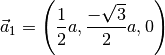
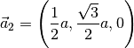
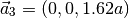
As an example, a hexagonal lattice could be input as:

1/2  -1/2   0      ! a1
1/2   1/2   0      ! a2
0.0   0.0   1      ! a3
6.2                ! lattice constant
0.0  -3.0  1.62    ! scale(1) is 1 by default

which corresponds to the lattice vectors (in Cartesian coordinates):

Atomic positions:

1. number of atoms in input (required)
2. For each atom: id pos1 pos2 pos2 (required) where id is an identifer (and default atomic number) and the atomic positions either in lattice or scaled cartesian coordinates (see &input ) Zero or more namelist(s) &origin can be inserted; all positions after that will have origin(:) added to each component
3. &shift shift(1) ... / (optional)Added shift to all atomic positions
4. &factor factor(1) ... / (optional) factor(s) to divide each component by
5. &gen or &sym (optional) symmetry given either by the generators of the group ( &gen ) or by all operations ( &sym )Next comes the information about the atoms . The id atomic identifer is used to relate the information to each atom; the default is to use id as the atomic number.
6. &allatoms (optional) information common to all atoms
7. &atom (optional) information for particular atomsThe rest of the input may be written to para or to inp.
8. For any other namelist see all parameters.; the order is generally not important. (optional)
9. &end (optional) stop reading the input; everything after this point ignored.

As an example of how easy/compact an input file can be, the following is all that is needed to run fcc Cu:

Cu (fcc)
&lattice bravais='cF' a0=6.50 /
   1                             ! number of atoms
   1    0   0    0
&atom     id=1  element='Cu'  /

Be aware that the defaults for k-points and iterations are probably not what you want, although the program will pick values that should give you a reasonable result. More commonly, one will give more information such as in this input:

GeMnN_2 (oP16 structure) (Antiferromagnetic)

&input cartesian=t checkinp=f /

   1     0     0
   0     1     0
   0     0     1
   10.367                 ! lattice constant
   1.0   1.2167  0.95625

   16                            ! number of atoms
    1  0.070   1/8   0
    1 -0.070  -1/8   1/2
    1  0.570   3/8   0
    1 -0.570  -3/8   1/2

    2  0.083  -3/8   0
   12 -0.083   3/8   1/2
   12  0.583  -1/8   0
    2 -0.583   1/8   1/2

    3  0.071   1/8   0.366
    3 -0.071  -1/8   0.866
    3  0.571   3/8   0.366
    3 -0.571  -3/8   0.866

    3  0.083  -3/8   3/8
    3 -0.083   3/8   7/8
    3  0.583  -1/8   3/8
    3 -0.583   1/8   7/8

&allatoms jri=361 lnonsph=4 dx=0.028 /
&atom     id=1  element='Ge' rmt=2.10 / ! econfig='[Ar] 3d10 | 4s2 4p1' /
&atom     id=2  element='Mn' rmt=2.20 /
&atom     id=12 element='Mn' rmt=2.20 /
&atom     id=3  element='N'  rmt=1.40 /

&comp gmax=12.0
      kmax=3.75
      jspins=2
/

&swsp 2=4 12=-4 /

&kpt  tkb=0.001 div1=8 kshift=t /
&mix  alpha=0.3 /

&conv itmax_scf=50  /

&geo l_geo=t maxstep=6 /

&out dosplot=t /

!&exco lda='pz'  /
 &exco gga='pbe' /

This sets up an antiferromagnetic system. Note that atoms with id=2 and 12 are the same; they are given different identifiers to force the symmetry program to treat them differently. The &swsp namelist starts the spin-polarized calculation with moments on atom with id=2 and 12. Note the use of comments in the input. At the end of the run, the density of states will be generated. Different choices for exchange-correlation are listed, but commented out, so the default will be used.