ANNOUNCEMENTS
MTH 437/537 — Spring 2019
- 6/17/19
-
The exams have been graded, and course grades assigned, although you may
not be able to see them until tomorrow.
The median score was 65 out of 80; the mean was 59.
-
You can collect your exam from me (and look at exam solutions) in my
office. I should be available most of this afternoon. After that,
check with me or stop by and take your chances — I do not keep a
regular schedule during the summer.
- 6/10/19
-
The final exam will be available for download
here
after 12 PM today.
-
You will need to provide a username and password, which will be sent to
your ONID email address this afternoon. If you have any difficulty
accessing the exam, please let me know.
- 6/5/19
-
The Sage notebook I demonstrated in class can be found
here.
-
This notebook uses the definition of the Kerr geometry that is built in
to Sage using a coordinate basis. A version using an orthonormal frame
can be found here, but Sage does not
seem able to compute the components of the Riemann tensor in a
reasonable amount of time using this method. It can, however, still
compute the connection, and verify that the Ricci tensor vanishes.
- 6/4/19
-
My office hours next week are listed below.
In most cases, the ending times will be extended if necessary to
accommodate those already present.
-
-
Monday, 6/10: 5–5:30 PM
-
Tuesday, 6/11: 1:30–4:30 PM
-
Wednesday, 6/12: 9:30–11:30 AM & 1:30–4:30 PM
-
Thursday, 6/13: 9:00 AM–12:00 PM
-
Other times may be possible, and I will also respond to email inquiries.
-
Please remember that you may not discuss any aspect of the exam
with anyone but me while you are waiting your turn.
- 6/3/19
-
Additional discussion of the
Standard Models
($\Lambda=0$) can be found in the text.
-
(Contrary to what was stated in class, these models do not
necessarily have $p=0$.)
-
We only discussed the first example ($p=0=k$) in class, known as
the Einstein–de Sitter cosmology.
-
A discussion of
cosmological redshift can also be found in the text.
- 5/30/19
-
My office hour tomorrow afternoon is again "preponed" by half an hour, and
will therefore be 1–1:45 PM.
- 5/29/19
-
The take-home final will be distributed online on Monday afternoon,
6/10/19.
It will be due in my office at noon on Thursday, 6/13/19.
-
-
The final covers Chapters 1–9 in the text.
-
It is fair to assume that all exam questions can be answered based on
mastery of the material we have covered in class.
-
Extensive office hours will be available during the exam.
-
You may use any non-human resources you wish, except
exam or homework solutions from previous years.
-
You may not discuss the exam with anyone other than me during
the exam period, even after you have turned it in.
- 5/26/19
-
I have set up an experimental interface to Sage
here that can in principle calculate
the connection 1-forms $\omega^i{}_j$, the curvature 2‑forms
$\Omega^i{}_j$, and the Ricci and Einstein tensors for any line element in
orthogonal coordinates.
-
Several examples have been implemented using this package, including
-
(There is also a partial verification of
Birkhoff's Theorem, which provides a
glimpse of the further capabilities of Sage.)
- 5/25/19
-
All indices can be raised and lowered with the metric.
-
For example, since $\TT=T^i{}_j\sigma^j\ee_i$, we have
$\ee_k\cdot\TT = T^i{}_j\sigma^j\ee_k\cdot\ee_i
= g_{ki}T^i{}_j\sigma^j = T_{kj}\sigma^j$
and similarly for $\RR$ and $\GG$.
- 5/24/19
-
I may be slightly late for my office hour this afternoon.
-
I am also available from 10–11 AM.
- 5/22/19
-
A discussion of Birkhoff's Theorem can be found in the
Appendix.
-
(There are minor typos in the Schwarzschild curvature 2-forms as given in
§A.3 of the text:
-
The coordinate expressions in the middle of Equations (A.52) and
(A.53) are each missing a factor of 1/2.
Also, the initial minus sign should be removed from Equation (A.61).
(The final expressions in terms of an orthonormal frame are correct.)
-
The
wiki version has been corrected, and a full list of errata
can be found
here.)
- 5/21/19
-
There are several computer algebra packages available for computing
curvature components:
-
-
A relatively recent option is to use the
SageMath cloud server;
see last term's announcements
dated 2/24/19 and 3/12/19.
-
One of the best has been the Maple package
GRTensor,
although I have not used the latest version, GRTensorIII.
-
Rough instructions on using the newer DifferentialGeometry
package, available in recent versions of Maple to compute curvature
tensors can be found here
-
Another option is the Mathematica code written to accompany Hartle's
textbook, which is available
online.
-
Finally, there is a fast but clunky LISP program
called SHEEP (aka CLASSI), which is available on the
ONID shell server, shell.onid.oregonstate.edu.
(See below for instructions.)
-
Printouts of (old!) sample computer algebra sessions are available for
GRTensor
and CLASSI.
-
Older versions of my instructions, that also include coordinate-based
computations, are available for
Maple and Mathematica packages,
and for SHEEP/CLASSI.
-
You may use software to compute curvature on the homework!
See me if you would like help getting started.
- 5/20/19
-
In addition to my usual WF office hours this week, I should be in my
office hour this afternoon from roughly 1:30–2:30 PM.
-
I am also available this morning, from roughly 10:30–11:30 AM.
- 5/19/19
-
In question 1b of HW 6, it is not necessary to
give an explicit formula for $g^{ij}$, although you may wish to do so in
the case of two dimensions. For the general case, a correct statement of
the system of equations, together with an argument as to why you expect a
unique solution, is sufficient, possibly accompanied by an interpretation
of these equations in terms of linear algebra.
- 5/18/19
-
As mentioned in class yesterday, I didn't get all the signs right for
expressions involving $\TT$.
(The energy density $\rho$ should be positive; the question in each
case is whether a given component is positive or negative.)
-
To the best of my knowledge, the signs in Chapter 8 of the text (which is
Chapter 7 of the wiki)
are correct.
-
In particular, the correct expression for observed energy density is
$\rho = +g(\TT,\vv\cdot d\rr)\cdot \vv = +T^i{}_j v_i v^j$.
- 5/17/19
-
My office hour this afternoon is "preponed" by half an hour, and is now
1–1:45 PM.
-
I am also available from 9–10 AM.
- 5/8/19
-
Here are the answers to the midterm questions:
-
-
(a) $-1$
(b) $-\left(1-\frac{2m}{r}\right)$
(c) $-1$
-
(a) $e=h(r)\dot{t}$
(b) $-\sqrt{\frac{2m}{r}-\frac{q^2}{r^2}}$
-
(a) Many answers possible, including $\rho=e^{\pm\alpha}$
-
(a) No
(b) $r=m\pm\sqrt{m^2-q^2}$
-
Worked solutions can be seen in my office, and will be discussed in class
on Friday.
- 5/7/19
-
The midterm has been moved to Bexl 417.
-
I should be in my office tomorrow (Wed) morning (roughly
10:30–11:45 AM) in addition to my office hour at 1:30 PM.
- 5/6/19
-
As discussed in class today, there are 10 independent Killing vectors in
4-dimensional Minkowsk space, namely 4 translations: $\xhat$,
$\yhat$, $\zhat$, $\Hat{t}$; 3 rotations:
$r\,\phat=x\,\yhat-y\,\xhat$, $y\,\zhat-z\,\yhat$, $z\,\xhat-x\,\zhat$;
and 3 boosts: $x\,\Hat{t}+t\,\xhat$, $y\,\Hat{t}+t\,\yhat$,
$z\,\Hat{t}+t\,\zhat$.
-
Each of these Killing vectors can be realized as coordinate symmetries
of the line element in appropriate coordinates, e.g. by switching to
round (spherical or cylindrical) or Rindler-like coordinates.
-
It is straightforward to show that each of the above vectors satisfies
Killing's equation, namely $d\XX\cdot d\rr=0$. Less obvious (but not
difficult to show) is that these are the only independent solutions
of that equation.
-
The collection of all Killing vectors forms a Lie algebra under
the operation of commutation, where vector fields act on each other by
differentiation. Lie algebras are infinitesimal versions of Lie
groups, representing continuous symmetries. For (some) further
information, see
Chapter 10 of our
octonions book.
- 5/4/19
-
A formula sheet will be available on the midterm. You can find a
copy here.
-
The current version is tentative; feel free to propose additions during
the review session on Monday.
-
I should be in my office most of Monday morning (roughly
9:30–11:45 AM) as well as before (roughly 12:45–2 PM) and
after class. I will also be in my office on Tuesday
(roughly 11 AM–2 PM, with a break for lunch);
(roughly 12:30–2 PM);
if you want to talk to me before 10 AM or after 2 PM you should contact
me in advance.
- 5/3/19
-
Further information about charged and rotating black holes and their
Penrose diagrams can be found in the undergraduate
textbook by d'Inverno, which is
on reserve.
-
A more advanced treatment can be found in the book The Large Scale
Structure of Space-Time by Hawking & Ellis, available in the
library.
- 5/1/19
-
The basis 1-forms $\sigma^T=dT$, $\sigma^R$ in rain coordinates are
defined in
§3.9,
but the rain cooordinate $R$ is not defined until
§A.4.
- 4/29/19
-
The midterm will be Wednesday 5/8/19 in class.
The main topics to be covered on the midterm are:
-
-
Line elements;
-
Spacetime diagrams;
-
Geodesics and their properties;
-
Schwarzschild geometry.
-
Further information:
-
-
The exam is closed book;
-
There will be a review during Monday's class.
Come prepared to ask questions!
-
A formula sheet will be provided, and will be discussed at the review.
-
I will hold extra office hours next week, most likely MW morning; other times
will be available by appointment.
- 4/28/19
-
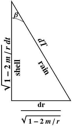
Figure 3.9 on page 38 (also available as Figure 8 in
this section),
showing the relationship between shell coordinates and rain coordinates, is
correct but misleading.
-
This figure shows the relationships between certain
differential forms, using the geometric description of
§13.8,
but without displaying the stacks. However, it is not easy in such
diagrams to read off the magnitudes of the differential forms, which do
not correspond directly to the lengths of the sides.
-
A more traditional figure, using the language of infinitesimal
displacement, is shown at the right.
-
Note added:
Spacetime diagrams implicitly show relationships between vectors.
For example, the figure at the right shows that
$$d\rr = \sqrt{1-\frac{2m}{r}}\,dt\,\Hat{t}
+ \frac{dr\,\Hat{r}}{\sqrt{1-\frac{2m}{r}}}
= dT\,\Hat{T}$$
if $dR=0$, that is, for a freely-falling object. Figure 3.9 shows
instead a relationship between 1-forms, namely that
$$1\,\sigma^T = \frac{\sigma^t}{\sqrt{1-\frac{2m}{r}}}
+ \frac{\sqrt{\frac{2m}{r}}\,\sigma^r}{\sqrt{1-\frac{2m}{r}}}$$
which is always true.
(The explicit inclusion of orthonormal basis 1-forms restores the proper
scaling to the triangle.)
- 4/15/19
-
The embedding diagram shown in class for the Schwarzschild geometry can be
constructed as follows.
-
-
Consider first a circle in the $(r,z)$-plane, with equation
$r^2+z^2=a^2$. The line element in the plane, restricted to the
circle, becomes
$ds^2 = dr^2+dz^2 = \left(1+\frac{r^2}{z^2}\right)\,dr^2
= \frac{a^2\,dr^2}{a^2-r^2}$.
-
More generally, if $z=f(r)$, then
$ds^2 = dr^2+dz^2 = \left(1+f'(r)^2\right)dr^2$.
-
Consider now the Schwarzschild line element, with $t$, $\theta$,
$\phi$ constant. The line element reduces to
$ds^2 = \frac{dr^2}{1-2m/r}$, so our goal is to find $f(r)$
so that $1+f'(r)^2=\frac{1}{1-2m/r}$.
-
Solving for $f'(r)$, we have first that
$f'(r)^2=\frac{2m/r}{1-2m/r}=\frac{2m}{r-2m}$, so that
$z = \int\frac{\sqrt{2m}}{\sqrt{r-2m}}dr = 2\sqrt{2m}\sqrt{r-2m}$,
or in other words $z^2+16m^2=8mr$.
-
Thus, $r$ is a quadratic function of $z$; the embedding diagram is a
sideways parabola, as displayed in class.
-
Do not forget that "$z$" does not exist! We can embed Schwarzschild
geometry in a higher-dimensional flat space, but we do not need to.
- 4/10/19
-
Breaking news:
See the first actual image of a black hole
here.
-
Also take a look here at today's
xkcd, showing just how large this black hole is.
- 4/10/19
-
Solutions of the geodesic equation in polar and spherical coordinates can
be found in
§19.5 and
§19.6.
-
The latter section also discusses using vector analysis to describe
arbitrary geodesics on the sphere.
-
You should check for yourself that $r\phat$ is indeed a Killing
vector, that is, that $d(r\phat)\cdot d\rr=0$.
-
Details can be found in
§2.2.
- 4/9/19
-
There will be no class on Friday, 4/12/19.
-
I encourage you to use this time – and the classroom – to
work jointly on the homework assignment due on
Monday.
- 4/8/19
-
We didn't quite finish deriving the geodesic equation on the sphere.
The answer can be found in
§19.3.
- 4/5/19
-
The schedule has been updated.
-
Among other things, the links for Wednesday and Friday of this week
were incorrect.
-
Figures for length contraction, which we discussed in class, can be
found
here.
-
The analogous figure for time dilation, which we did not discuss,
can be found
here.
- 4/3/19
-
As mentioned in class today, the sets of spacelike, timelike, and
lightlike vectors do not close under addition (even with the zero vector
included), and thus do not form a vector space.
-
Can you find counterexamples?
-
However, the set of future-pointing (or past-pointing) timelike
vectors do close under addition (with the zero vector included), and
therefore do form a vector space.
- 4/2/19
-
My office hours have now been posted on the
course homepage.
-
I am often in my office MWF mornings from roughly 10–11:30 AM, and
am also usually available after class. Feel free to drop in at those
times — or to contact me to arrange an appointment at these or
other times.
-
My rough schedule can be found
here.
- 4/1/19
-
As discussed in class today, I propose an extra, optional meeting to go
over the final from last term.
-
This session is tentatively scheduled for
this Friday, 4/5/19, at 2 PM in
our regular classroom (Bexl 323)
Bexl 320.
- 3/30/19
-
The primary text for this course will be my own
book,
which can be read online as an
ebook
through the OSU library.
-
There is also a freely accessible
wiki
version available, which is however not quite the same as the
published version.
-
We will also refer briefly to my
book on special relativity.
-
You may purchase this book if you wish, but it can also be read online as an
ebook
through the OSU library, and again there is also a
wiki version.
-
You may also wish to purchase a more traditional text, in which case I
recommend any of the first three optional texts listed on
the books page. The level of this course will be
somewhere between that of these books, henceforth referred to as EBH
(Taylor & Wheeler), Relativity (d'Inverno), and Gravity
(Hartle).
-
-
EBH uses only basic calculus to manipulate line elements, and only
discusses black holes, but does so in great detail.
-
Relativity discusses the math first, then the physics.
-
Gravity begins essentially the same way, starting from a given line
element to discuss applications, including both black holes and other topics.
This is followed by a full treatment of tensor calculus, including a
derivation of Einstein's equation. This book is the most advanced of the
three, and is aimed at advanced undergraduate physics majors.
-
We will cover more material than EBH, but we will stop short of the
full tensor treatment in Relativity or (the back of) Gravity.
We will also cover some of the material on black holes from EBH which
is not in Gravity or Relativity.
-
-
If you are seriously interested in the physics of general relativity,
Gravity is worth having.
-
If you are primarily interested in the mathematics, you may find
Relativity easier to read. It covers more topics more quickly
than Gravity.
-
However, we will use the language of differential forms wherever we can, which
is not extensively covered in any of these other books. We will therefore
take a somewhat more sophisticated approach than EBH, while trying to
avoid most of the tensor analysis in Gravity or Relativity.
-
In short, none of these books is perfect, but all are valuable resources.
In addition to the above books, OSU owns an electronic copy of
Relativity Demystified,
which summarizes many of the key aspects of relativity, but provides no
derivations. By all means use it for reference, but I would not recommend
using it as a primary text.