The problem of determining the maximum or minimum of function is encountered in geometry, mechanics, physics, and other fields, and was one of the motivating factors in the development of the calculus in the seventeenth century.
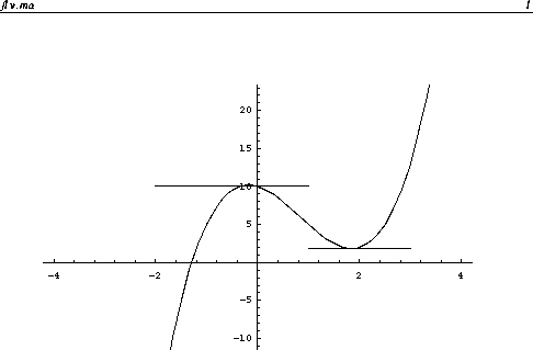
Let us recall the procedure for the case of a function of one variable y=f(x). First, we determine points x_c where f'(x)=0. These points are called critical points. At critical points the tangent line is horizontal. This is shown in the figure below.
The second derivative test is employed to determine if a critical point is a relative maximum or a relative minimum. If f''(x_c)>0, then x_c is a relative minimum. If f''(x_c)<0, then x_c is a maximum. If f''(x_c)=0, then the test gives no information.
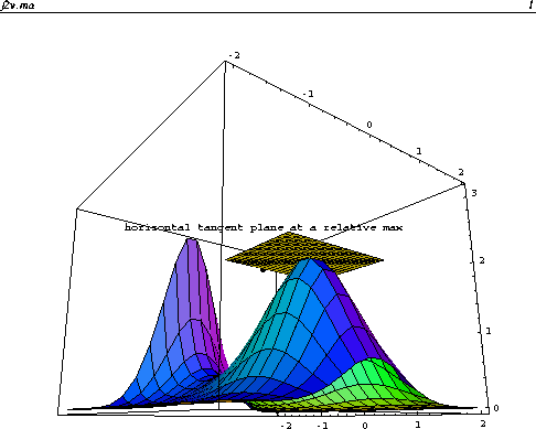
The notions of critical points and the second derivative test carry over to functions of two variables. Let z=f(x,y). Critical points are points in the xy-plane where the tangent plane is horizontal.
Since the normal vector of the tangent plane at (x,y) is given by
![]()
The tangent plane is horizontal if its normal vector points in the z direction. Hence, critical points are solutions of the equations:
![]()
because horizontal planes have normal vector parallel to z-axis. The two equations above must be solved simultaneously.
Example
Let us find the critical points of
![]()
The partial derivatives are
![]()
![]()
f_x=0 if 1-x^2=0 or the exponential term is 0. f_y=0 if -2y=0 or the exponential term is 0. The exponential term is not 0 except in the degenerate case. Hence we require 1-x^2=0 and -2y=0, implying x=1 or x=-1 and y=0. There are two critical points (-1,0) and (1,0).
The Second Derivative Test for Functions of Two Variables
How can we determine if the critical points found above are relative maxima or minima? We apply a second derivative test for functions of two variables.
Let (x_c,y_c) be a critical point and define
![]()
We have the following cases:
An example of a saddle point is shown in the example below.
Example: Continued
For the example above, we have
![]()
![]()
![]()
For x=1 and y=0, we have D(1,0)=4exp(4/3)>0 with f_xx(1,0)=-2exp(2/3)<0. Hence, (1,0) is a relative maximum. For x=-1 and y=0, we have D(-1,0)=-4exp(-4/3)<0. Hence, (-1,0) is a saddle point.
The figure below plots the surface z=f(x,y).
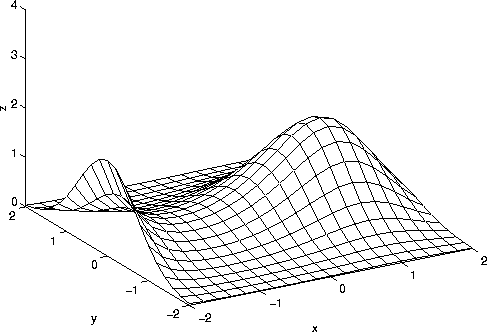
Notice the relative maximum at (x=1,y=0). (x=-1,y=0) is a relative maximum if one travels in the y direction and a relative minimum if one travels in the x-direction. Near (-1,0) the surface looks like a saddle, hence the name.
Maxima and Minima in a Bounded Region
Suppose that our goal is to find the global maximum and minimum
of our model function above in the square -2<=x<=2 and
-2<=y<=2?
There are three types of points that can potentially be global
maxima or minima:
We have already done step 1. There are extrema at (1,0) and (-1,0). The boundary of square consists of 4 parts. Side 1 is y=-2 and -2<=x<=2. On this side, we have
![]()
The original function of 2 variables is now a function of x only. We set g'(x)=0 to determine relative extrema on Side 1. It can be shown that x=1 and x=-1 are the relative extrema. Since y=-2, the relative extrema on Side 1 are at (1,-2) and (-1,-2).
On Side 2 (x=-2 and -2<=y<=2)
![]()
We set h'(y)=0 to determine the relative extrema. It can be shown that y=0 is the only critical point, corresponding to (-2,0).
We play the same game to determine the relative extrema on the other 2 sides. It can be shown that they are (2,0), (1,2), and (-1,2).
Finally, we must include the 4 corners (-2,-2), (-2,2), (2,-2), and (2,2). In summary, the candidates for global maximum and minimum are (-1,0), (1,0), (1,-2), (-1,-2), (-2,0), (2,0), (1,2), (-1,2), (-2,-2), (-2,2), (2,-2), and (2,2). We evaluate f(x,y) at each of these points to determine the global max and min in the square. The global maximum occurs (-2,0) and (1,0). This can be seen in the figure above. The global minimum occurs at 4 points: (-1,2), (-1,-2), (2,2), and (2,-2).
Example: Maxima and Minima in a Disk
Another example of a bounded region is the disk of radius 2 centered at the origin. We proceed as in the previous example, determining in the 3 classes above. (1,0) and (-1,0) lie in the interior of the disk.
The boundary of the disk is the circle x^2+y^2=4. To find extreme points on the disk we parameterize the circle. A natural parameterization is x=2cos(t) and y=2sin(t) for 0<=t<=2*pi. We substitute these expressions into z=f(x,y) and obtain
![]()
On the circle, the original functions of 2 variables is reduced to a function of 1 variable. We can determine the extrema on the circle using techniques from calculus of on variable.
In this problem there are not any corners. Hence, we determine the global max and min by considering points in the interior of the disk and on the circle. An alternative method for finding the maximum and minimum on the circle is the method of Lagrange multipliers.
Maxima and Minima for Functions of More than 2 Variables
The notion of extreme points can be extended to functions of more than 2 variables. Suppose z=f(x_1,x_2,...,x_n). (a_1,a_2,...,a_n) is extreme point if it satisfies the n equations
![]()
There is not a general second derivative test to determine if a point is a relative maximum or minimum for functions of more than two variables.
[Vector Calculus Home] [Math 254 Home] [Math 255 Home] [Notation] [References]
Copyright © 1996 Department of Mathematics, Oregon State University
If you have questions or comments, don't hestitate to contact us.