![]()
![]()
 and
Hans Kowallik
and
Hans Kowallik
rubin@physics.orst.edu
http://www.physics.orst.edu/~rubin
Applying computer technology is simply finding
the right wrench to pound in the correct screw. -Anonymous
In this paper I wish to describe and demonstrate the Web-enhanced Computational Physics book and course we have developed in the Physics Department of Oregon State University. By the end of the paper I hope you will agree that the integration of the course, textbook, and Web tutorials produces a new and effective approach for education and publishing. The course is intended for upper-level undergraduates or beginning graduate students, and the book, Computational Physics, Problem Solving with Computers,[1] containing all the projects for the course, is enhanced by links to free, interactive Web tutorials containing sonifications, animations, and JAVA applets.
We have developed the course and written the text over a seven year period with support from the U.S. Department of Energy, the U.S. National Science Foundation, and IBM. The Web materials were developed in the last three years with initial support from the Undergraduate Computational Engineering and Science project (UCES)[2], and with sustained support from the Northwest Alliance for Computational Science (NACSE)[3]. This last organization is an NSF Metacenter Regional Alliance which strives to exploit Web technology to improve the use of high performance computing (HPC) resources in science and engineering.
While some of the Web materials are directly related to the course, others are more general, dealing ideal with visualizations, HPC library use, PVM, and Coping with Unix (both a real book [4] and Web tutorials[5]). Accordingly, the Web materials can be used in the traditional University and High School education settings, or in a scientist's and engineer's workplace.
This package of educational materials is not what I planned on writing when, about a decade ago, I started the discussions that led to our Computational Physics course. I though the Computer Science Department would teach the students what they needed to know about computers, the Mathematics Department would teach them what they needed to know about numerical methods and statistics, and I would teach them how to apply that knowledge to solve physics problems using computers. That's how I thought it would be. But, by and large I have found that the students taking the Computational Physics course do not carry the subject matter from these other disciplines with them. And so a lot of what we have put into the material we developed would, in a more perfect world, be taught and written by experts in these other fields.
While that is why I feel this is not the material I thought we would be developing, I believe it's probably for the better. On the one hand, having a basic research physicist tell students they need to know "this" in computer science and "that" in mathematics, gets the message across that "this stuff really matters". On the other hand, it is useful to have the physics, mathematics, and computer science concepts conveyed in the language of a natural scientist and within the context of solving a problem scientifically.
I believe that our work is an excellent example of that interdisciplinary mixture of computer science, mathematics, and discipline (in our case physics) that is known as "Computational Science". While much of what we hear about computational science education deals with what computer science should be taught to science students, I believe that computational science education needs to focus more on its science and applications in order for the field to be vital.
As a case in point, I have tried to make computational science education become alive for students by having the clever, but transparent, use of computers stimulate their innate intellectual interest in understanding and finding beauty in the world in which we live. The critical element here is that the computer is truly an excellent tool for amplifying our cognitive and reasoning abilities. In my way of thinking, there is nothing like having your science, be it some mathematical equations and lines of code, or some abstract connection among ideas, come alive right before your own eyes actually looking like the real world. After that type of "close encounter", students often go back to learn more of the underlying science and more powerful tools in order to understand better what is happening. I find that teaching gets to be much easier once students are motivated, are interacting with the materials, and are doing it all without too much pain.
The educational material we developed is in the form of individual projects, each of which follows a problem-solving paradigm of the type developed by the UCES[2]:
Figure 1: The UCES or "problem solving" paradigm.
This paradigm clearly distinguishes the different steps in scientific problem solving, the use of the best or the available tools, and the value of continual assessment (the double-headed arrows). It also makes it clear that computational science is an interdisciplinary field founded on the scientific process.
The course differs from many others in its underlying philosophy:
I hear and I wonder,
I see and I follow,
I do and I understand.
-as recalled from a fortune cookie
The specific objectives of the course are:
The projects are designed to help students learn by having them solve a very wide class of problems employing differing scientific, mathematical, and computational techniques. As a consequence of having to interact with the material and having to understand it in order to get their problem solved, the material becomes part of the personal experience of the students. In this way the students are often stimulated to learn more about these subjects, or to listen more closely when they are covered in other courses. Although the majority of my students have come from physics, there is also value in teaching the problem-solving approach to computer science students; in this way the latest programming paradigms can actually encounter realistic applications.
For example, I have heard students comment that "I never understood what was dynamic in thermodynamics until after this simulation," and "I would never have imagined that there could be such a difference between upward and downward recursion," as well as "Is that what a random walk really looks like?" or "Why is the pendulum jumping around like that?" In my experience, a teacher just does not hear students express such insight and interest in course material in a standard lecture course.
When we first started teaching this course, which typically contains 10-20 students, we envisioned that the students would read the assigned materials before hand and then work through the projects in the computer lab with the help of the professor and teaching assistant. Possibly as a consequence of the newness of much of the material, or of the breadth of the subjects covered, there has been a uniform desire on the part of the students to have some traditional style lectures as part of the course. It seems important to give a broad picture of the material and to make it clear what is expected of the students in their projects. It is interesting that this does not agree with the vision of education administrators who no longer sees professors at the front of a class when computers and the Web are used in education.
The course and book materials divides into five parts which we cover, pretty much, in order. Here are the Parts with with local links to chapters and sections:
There is a price to pay for the unusually broad approach we see with all these topics: the students must work hard and cannot master material in great depth. The workload is lightened somewhat by providing "bare bones" programs, and the level is deepened somewhat by having references and Web tutorials readily available. By eliminating time-consuming theoretical background more properly taught in other places, and by deemphasizing timidity-inducing error analysis in every single procedure, the students get many of these challenging projects "to work" for them and enjoy the stimulation of experiencing the material. In the process, the students immediately gain pride and self-confidence, and this makes for a fun course for everyone.
The first quarter of the course concentrates on the basic mathematical, numerical, and conceptual elements needed for using computers as virtual scientific laboratories. We start off slowly, in part because this is the first experience some students have with Unix. After learning about Unix systems, we study the basics of computing: algorithms, precision, efficiency, and verification, and then move on to some numerical analysis and associated approximation and round-off errors.
Learning Unix is less of a problem than it used to be, because our NACSE[3] group has taken a conventionally-published Guide for Scientists and Engineers[4] and used it as a base for a series of Interactive Unix Tutorials[5]. The Unix tutorials use some Java-based Web technology (Webterm) we developed which makes it possible for a browser to connect to a remote Unix machine and execute Unix command - even browsers on non-Unix computers such as PCs or Macs. Many students take the tutorials their own either before or during the course.
The second quarter focuses on realistic physical problems which apply and extend the preceding techniques. (There are more applications than can be studied in one quarter, and so some customizing is made to each student's interests.) An important aspect of the course is the use of advanced library routines, multiple-subroutine programs, interactions with larger research codes, and the use of supercomputers or parallel workstation clusters. This is often the only place students experience these common aspects of computational science.
After discussions with an instructor, each student writes up each project as an "executive summary" focusing on
The emphasis is to make the report an executive summary of the type given to a boss or manager; just tell enough to get across that you know what you are talking about, and be certain to convey what you did and your evaluation of it. Recently, some students have written their reports as hypertext documents for the Web, an ideal environment for computational projects with the projects always in a centralized place for the students and faculty to observe, the original code there to run or modify, and the visualizations striking in 3-D color or animation (examples to follow).
An unusual aspect of our Computational Physics textbook is that to an increasing degree we are enhancing it with interactive tutorials available free on the World Wide Web. This is now a NACSE[3] research project aimed at better incorporating high-performance computing techniques into science and engineering. Following the Web links in the Contents leads to full listings of all sections in the book and then to Web enhancements such as running codes, figures, animations, sonifications, corrected code listings, and control-panel interfaces. While these are not meant to be a substitute for studying the text or running one's own codes, they do provide prototypes of what can de done and how the physics can be "seen" in differing ways (such as seeing phase space plots drawn as a pendulum swings, or hearing the noise made by a chaotic pendulum).
For example, for Chapter 6 you find:
Chapter 6: Deterministic Randomness
(Web links)
Enough of words. To get a feel for how the science and computation strengthen each other, we look at some examples.
In Figure 2 we see seven 2D random walk simulations from
a student's report [6] on the Monte
Carlo project. Each walker takes 1000 steps starting at the origin. The
data were produced by the program (Web link) walk.c.
Although random processes are discussed in many undergraduate science and engineering courses, it is surprising to learn how few students have ever seen one! They often ask me if their results are correct - as if being a physics professor gives you the ability to see molecules collide. I tell them that if their computer simulation yields predictions which agree with experiment, then it is likely to have some truth in it. In some sense, then, they are "seeing" a random walk.
Figure 2: Seven random walks starting from the origin.
By uncovering correlations in pseudorandom number, the
students have already seen that the random number generators are not truly
random and so know to suspect Monte Carlo simulations. To check the validity
of models of random processes, in Figure 3 we give results from a student's
project for the distance covered after N random steps versus ![]() .
.
Figure 3: The distance R from the origin after N two-dimensional
random steps. The dashed curve is the theoretical results, the red and
black solid curves correspond to different algorithms for choosing random
steps in two dimensions.
We see that although the theory of random processes predicts that for large N,
where ![]() is the square root of the average squared step size, this holds only on
the average after many trials, and even then only if particular care is
used in generating the random walk (the different curves in Figure 3).
is the square root of the average squared step size, this holds only on
the average after many trials, and even then only if particular care is
used in generating the random walk (the different curves in Figure 3).

In Figure 4 we present the results of a Monte-Carlo simulation
of radioactive decay (spontaneous emission). The simulation is based on
the basic, phenomenological fact of decay: for ![]() particles at time t, the number of these particles decaying in some
small time interval
particles at time t, the number of these particles decaying in some
small time interval ![]() is proportional to both the number of particles present N, and the
length of the time interval:
is proportional to both the number of particles present N, and the
length of the time interval:
This leads to the basic algorithm for each nucleus:
if ![]() , the nucleus decays and Nnuc=Nnuc-1; else it remains.
, the nucleus decays and Nnuc=Nnuc-1; else it remains.
Figure 4: Simulation of the Spontaneous decay of 1000 and 10 atoms
with a decay constant of 0.1. The black curve only "looks" exponential,
it is actually stochastic.
The results in Figure 4 are of a simulation of this equation. Notice that for N=1000 the curve starts very smoothly, but becomes more steplike as the number of atoms decreases. These simulations show the student that the decay rate (the slope of the curves) is independent of the number of initial nuclei (the curves are scaled to begin at the same point). Of even more interest, the student sees that for large numbers of nuclei, the decay can be approximated well by an exponential (a straight line on this semilog plot), but that for small N, the process is stochastic in nature.
These simulations shatters the student's prejudice that the analytic result (exponential decay) is "exact" while the computed model is a less accurate description of nature. Here the numerical simulation holds for all values of N, while exponential decay clearly becomes a poorer and poorer approximation as N decreases (which of course is what always happens eventually in nature).
The student's belief in the decay simulation and their
understanding of nature is further strengthen by our Web Geiger-counter[8].
This enhancement converts a numerical N versus t graph into
a series of 1's and 0's, opens up a sound player, and then "plays"
the decay simulation. For example, here you can hear (beware, you need
a sound player to hear it) the sounds of decay(.au
8k). It is important to note that you are hearing a simulation
produced by equations and not the recording of a real Geiger counter. Listen
and see if you can hear the decay change from exponential to stochastic
as nuclei decay.
Here is a sample (CGI-bin scripts over the Web) of the interface to our Web Geiger counter. You hear it measure the radioactivity of a sample after specifying the decay rate and the number of initial nuclei. To keep the size of the sound file and the amount of CPU time on our machine reasonable, we have limited the maximum number of atoms to 500 and the length of the sound files to 10 seconds.
First we look at some examples from a student's project[6] on the chaotic pendulum. The angular form of Newton's laws of motion, including a periodic driving force, viscous damping, and a nonlinear restoring force proportional to the sine of the angle of displacement, are:
In Figures 5 and 6 we show some animated gif solutions of these equations:
Figure 5: Left: A model of a chaotic pendulum; Right: The angular
displacement of the pendulum versus time. The red vertical line shows the
current angular position of the pendulum (push "Reload" to reanimate
the pendulum).
Figure 6: Left: A model of a chaotic pendulum; Right: A phase space
plot (angular velocity versus angular displacement). The red vertical line
shows the current position and velocity of the pendulum (push "Reload"
file to animate).
Actually, we have developed a number of Web tutorials on this topic,[3] but the reader really needs to look at them over the Web to appreciate them. Our most recent are JAVA applets which permit interactions, very fast (local) animation of a variety of chaotic behaviors, and some research-level studies of the levels of complicated behavior. A snapshot of one of these applets is shown in Figure 7. The actual applets (which may require you to change the .CLA file extensions to .class ones) are:
The buttons are used to start, stop, and clear animation (before rerun), and the possible configurations listed can be chosen with mouse clicks. In Figure 7 or the applets, you can see how all the parameters can be easily adjusted and how a comparison can be made of two chaotic pendula with slightly differing initial conditions.
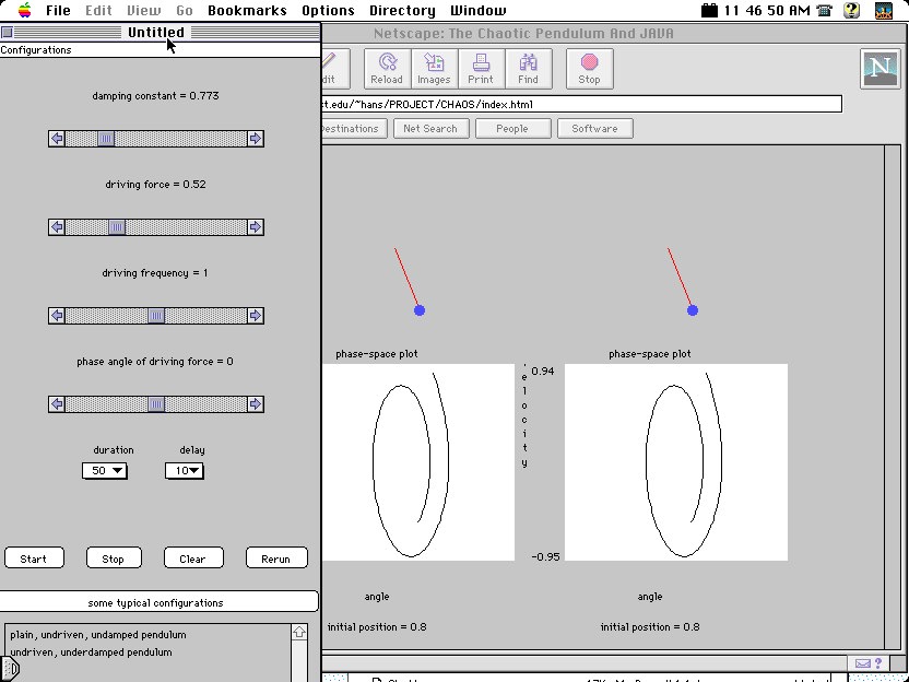
Figure 7: A snapshot of a Java applet showing the control panel
on the left and the comparison of two animated pendula and their phase
space plots.
These animations and applets show how multimedia can help students learn some difficult and abstract concepts. On the one hand, the picture of a pendulum actually swinging is a concrete example of chaotic motion with its combination of oscillations with multiple periods and "over the top" rotations. Seeing this motion occur as the displacement versus time graph is being drawn, breathes life into what otherwise appeared like just a graph. Seeing the phase space plot being drawn along with the other plots adds meaning at different levels of understanding to what is otherwise an abstract concept. Since modern dynamics is greatly simplified by viewing it as geometry in phase space,` these visualization help the student make that transition to a simple, yet more abstract, viewpoint.
Figure 8: A high school statics problem showing two masses suspended
by three strings.
Below (in small print) we give some pages from a Web tutorial we originally developed for a high school physics class and now have use in our course. The physics problem is a simple one from statics in which there are two weights hanging from three strings of known lengths, and you are asked to determine the angles of and tensions in the strings (for graduate work we like to increase the number of weights).
This is a great problem for computational science because it is easy to write down the equations which need to be solved, and even though there is no helpful analytic solution, they do have an easy numerical one ("easy" if one uses a scientific subroutine library). In addition, the student can interact with the material by running "experiments" (different parameter choices), and trying to make the computer "fail". As the student looks into the details of the problem, she sees that the numerical approach is based on a search procedure which succeeds only if a physically-reasonable initial guess is made. Accordingly, the student sees that the computer may be the only way to solve even some simple problems, although there is still a critical need for human insight and intuition.
When you press the "Find Solution", the numbers
in the form are sent back to our computer in the Department of Physics
of Oregon State University, and a Fortran
program is executed on a high performance computer. If all goes well,
you should get the answers back after waiting a while. Go ahead and try
it!
We have already discussed and heard in this paper the Web Geiger counter which, by "playing" decay simulation data, sounds like a real Geiger counter. In addition to that, we have developed tutorials[10] which investigate other ways in which sound can be used to visualize, or more properly, "sonify", physical phenomena. For example, the physics and mathematics used to describe harmonic, anharmonic, and chaotic oscillators come alive when students can hear them.
I believe sonification assists the learning process by adding senses other than sight to it. Another consequence of sonification is that it makes science more accessible to the print disabled (the blind). In fact, our collaboration with the Science Accessibility Project[11] has verified that this conclusion holds equally well in reverse: by making science more accessible to the print disabled, we improve the learning for sighted students as well. Accessibility is clearly a valuable and need-to-be developed use of the Web. As a case in point, the figures and gif-formatted equations we show also contain text descriptions in the ALT= HTML tag, and this provides useful information for people, or browsers, that cannot view images.
We present here (with local links for sound players) some sonification tutorials which explore methods of creating sound files to represent physical systems.
This is the simplest case in which we convert data directly into a format which can be used by a soundplayer. As the output varies, so does the sound:

Figure 9: One cycle of the angular position versus time for a realistic
(not small angle) pendulum. The full signal is periodic and repeats indefinitely.
Selecting this image will play a 35K sound file of this signal.

Figure 10: One cycle of the position versus time for an anharmonic
(nonsinusoidal) oscillator. Selecting this image will play a 40K sound
file of this signal. Listening to it, you should note more overtones (higher
harmonics) than in the preceding pendulum, that is, a fuller or less simple
tone.

Figure 11: The nearly chaotic motion of a ball driven by an external
sinusoidal force but constrained to move within a box. Selecting this image
will play a 35K sound file of this signal. Do not try to fix your sound
player, this signal should sound "noisy" because there
are a number of frequencies occurring sequentially.
Figure 12: The bifurcation plot of the logistics map. Selecting
this image will play a 204K sound file in which each bifurcation is represented
by a tone proportional to its height.
In Figure 12 we have the familiar bifurcation plot (bug population versus growth rate) of the logistics map with its continuous series of bifurcations. To visualize this plot with sound, we interpret it as a Fourier spectrum with the growth rate (abscissa) the sound frequency and the population (ordinate) as the sound amplutide. When there is only one population, there will be just one frequency played, yet the frequency will increase as the population increases. When there are two populations, there are two frequencies played. And when there is chaos, many frequencies are played. In fact, there is at least some poetic justice here since chaotic motion is the combination of many of periodic motions; as we hear the sound recording progress from chords to noise, we are hearing the system progress from complicated behavior to chaos.
We have developed a university-level course in Computational Physics, a book based on this course, and an extensive collection of Web tutorials to enhance the book and course. The tutorials are multimedia, interactive, and free. My aim was not just to teach the use of computers in physics education, or to teach physics with computers, but rather to see computational science become a more significant part of university education.
After observing the kinds of materials that are out there on the Web, I have concluded that if Web material is to have a significant impact on education, then it needs to be presented as part of a coherent, organized body of knowledge (this is the logic behind us developing a course-book-Web tutorials package). Even with the latest technologies, conventional books are still valuable. They
As a package, the material does appear to work well together, yet our student feedback informs us that there is still much value in having a Professor give lectures in front of a class.
The prerequisites we initially established for our course included programming experience in a compiled or symbolic language, numerical methods, and mathematical methods of physics including statistics, data fitting, and linear algebra. Unfortunately, I have had to relax these prerequisites since so few of our students could meet them (a condition which is only getting worse as universities compete for students with each other by lowering the number of credits needed to graduate).
Even though most students have taken some computer science courses, I have found that our course often serves as the students' first introduction to scientific computing; this means there is less time to do science on the computer and to experiment. We have tried to alleviate this shortcoming by collecting some needed background into a Guide For Scientists And Engineers[4] and Web tutorials [5] based on that guide. I have also helped introduce an Introduction to Scientific Computing course for students at the freshman or sophomore level; this should leave more time for science in upper-level courses.
The reviews for the course have been uniformly high, even though working through the large number of projects and the requisite programming skills are a challenge for students. In some cases these challenges have been overwhelming. I personally have been rewarded in this course by a level of discussion rarely encountered in other courses and with students actually asking for additional materials. The project approach proves to be flexible and to encourage students to take pride in their work and their creativity.
The availability of tutorials and auxiliary materials on the Web have made us more efficient when teaching the course. The animations and sonifications available to the student have extended and possibly deepened their education. In this way the Web certainly makes learning more engaging and easier. On the teacher's part, the investment in time to develop and maintain the materials is tremendous, and has only been possible through the hard work of graduate students and staff, and the support of research grants.
Some of our students have gone on to study computational science at summer schools, some have made it a career option in graduate school, and others have found the projects and scientific computing experience useful in their employment. For sure, it's been exciting to teach.
We have benefited from support from the U.S. National Science Foundation (curriculum Development grant), the U.S. Department of Energy, the Undergraduate Computational Engineering and Science Project (who gave RHL an award for the course development), and the NSF's Northwest Alliance for Computational Science (NACSE). The tutorials have benefited from the work of Jon Maestri, Melanie Johnson, Paul Hillard, and Kevin Wolver. Helpful discussions with Cherri Pancake, Henri Jansen, Pat Canan, Al Wasserman, Ken Ferschweiler, and John Reed are gratefully acknowledged.
Rubin H Landau is a professor of physics at Oregon State University. In the past he has held positions at IBM Research, the Weitzman Institute of Science, the San Diego Supercomputer Center (NPACI), the Institute for Nonlinear Science (UCSD) and the Universities of British Columbia, Pittsburgh, Surrey, Melbourne, Adelaide, and California (Berkeley and San Diego). He has a Ph.D and an M.S. from the University of Illinois, and a B.S. from Cornell University. Landau's research interests are in the theory and computation of few body systems of elementary particles and quarks, computational physics, and computational science education. He is the author or coauthor of some 80 scientific publications, as well as several books published by John Wiley: Quantum Mechanics II; A Scientist's and Engineer's Guide to Workstations and Supercomputers, Coping with Unix, RISC, vectors and programming; and Computational Physics, Problem Solving With Computers. Landau is a member of the American Physical Society, the IEEE Computer Society, the American Association of Physics Teachers, Sigma Xi, and the American Association of University Professors, and has held offices or served on committees in several of these organizations.
 ,
,