Table of Contents

• Announcements
• Introduction
• Basic Python Programming
• Read About Instrumentation Communication
• Learn About the Oscilloscope and Function Generator
• Communicate With The Oscilloscope
• Analyze and Rewrite the Initialization Program
• Investigate the Ohmic Behavior of a Resistive Potential Divider Using Marina

Announcements

• Confirm that the most recent versions of the following Python software packages are available on your computer. If not, then log in and download the newest versions by clicking on View Files and following the Python path to the zip files:
  • Marina
  • Measure the transmission function A(ω) of a circuit using scan_2.py.
  • Simulate the response A(ω) of a circuit using simulatem.py.
  • Plot the simulations, data and both together using response_plot.py.

Introduction

• This task will introduce programming with Python, communicating with USB-based instruments and simple signal processing.
• The experiments are the following: I(V) response of a purely resistive object; complex impedance spectrum of an object.

Basic Python Programming

• Open a DOS session and run the command "python". Follow the programming instructions.
• From start menu -> python, run Idle, a simple IDE, and follow the programming instructions.
• From the start menu, run geany, a real IDE for several programming languages and even LaTeX. Compose and execute simple programs outlined by the instructor.
• On the Python Wiki site, go to the "Basics" page and experiment with the programs.
• Copy and execute the simple plotting program provided by the instructor to generate a data set using the numpy module and plot it using the pylab module. The pylab module is part of the matplotlib package which provides Matlab style graphing functionality. Read the Python page for more information.

Read About Instrumentation Communication

• Peruse the entire instrumention page.
• Visit the PyVisa site and read the documentation.
• Peruse the Standard Commands for Programmable Instruments (SCPI) document.

Learn About the Oscilloscope and Function Generator

• Familiarize yourself with the printed operation manuals for the TDS1012B oscilloscope and the AFG3021B function generator.

Communicate With The Oscilloscope

• On the oscilloscope page, read about the programming syntax.
• Follow the "detecting and initializing" instructions.
• Follow the "capturing and plotting waveforms" instructions.

Analyze and Rewrite the Initialization Program

• Analyze the initialization suite of programs in writing. Specifically: find all objects and list the attributes and functions; find all functions and list the input requirements and returned quantities; draw a flow diagram at the object and function level describing the operation of the program; list all instructions sent to both instruments.
• Write a new parameters file to set the function generator to provide a bipolar ramp at 100 kHz with V_pp = 2 V into 1 MΩ. Set the oscilloscope to display white on black, channel 1 for 3 V_pp full scale, 3 cycles across the screen and averaging over 64 waveform acquisitions.

Investigate the Ohmic Behavior of a Resistive Potential Divider Using Marina

• Build a simple resistive divider with identical resistors and apply a bipolar ramp from the function generator. Set the output impedance value on the function generator to the correct value. Connect this signal to channel 1 of the oscilloscope and the signal across the resistor to channel 2. Use DC coupling. Set the frequency to 100 Hz and the amplitude to 1.0 V.
• Set the oscilloscope to display two ramp cycles, with both waveforms scaled to use the entire dynamic range of the ADC (the entire vertical range of the display).
• Run marina by executing control.py in your Marina application directory. Select the oscilloscope on the hardware tab and acquire a waveform on the waveform acquisition tab. Generate a graph of V₂(V₁) and save the data as a csv file. Do this also for 5 V at 100 Hz and 5 V at 250 kHz (the maximum ramp frequency). Finally, try a 5 V sinewave at 10 MHz. Explain any observed phase shift in terms of a specific model of passive components for your experimental arrangement and discuss the effect on your ability to determine Ohmic behavior.
• Download plot.zip, and use response_plot.py to make plots of data stored in a csv file. The program is set to run example 7 using the data set xy.csv which is an xy data set acquired from the oscilloscope by scope_waveforms.py.
• Determine the validity of the assumed Ohmic behavior of the resistors under test. Fit a straight line indicative of Ohmic behavior to V₂(V₁). The program polyfit_fit.py on the Python page demonstrates how to use numpy to fit polynomials to data and to use the residuals as a measure of the certainty of the fit. To fit a polynomial to an approximately linear set of data in a csv file created by scope_waveforms.py or scan_2.py, use fit_linear_data_bins-corrected.py. Note that you must specify the name of the file and the arrays to be used in the Test() routine. 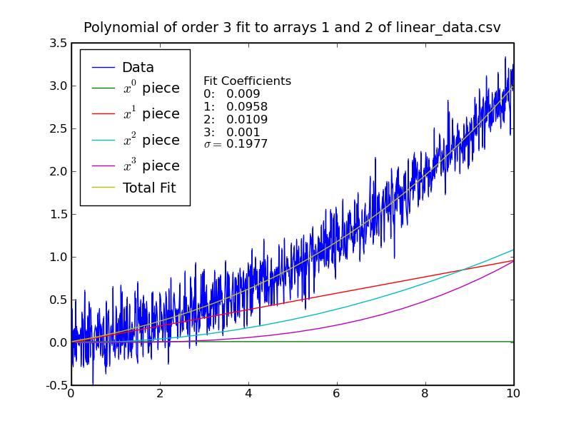A sample csv file is linear_data.csv, which was generated by make_linear_data.py
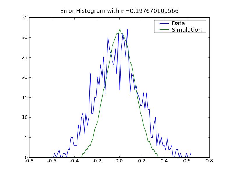
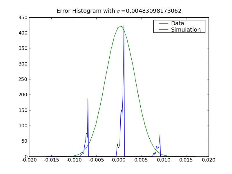
• Graphs of linear_data.csv: polynomial fit error histogram.
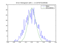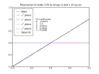
• Graphs of xy.csv: polynomial fit error histogram.
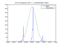• Use the error histogram plotting capability of fit_linear_data.py to analyze the noise distribution of V₂(V₁). Note that the program also graphs the normal gaussian error function of the same σ. Explain the interesting experimental error distribution for the digitized data from the scope as in the analysis of xy.csv above. Consider that the oscilloscope performs 8 bit analog to digital conversion (ADC). The entire vertical range is then reduced to only 256 possibilities, from 0 to 255. As can be seen in scope_waveform.py, the waveform acquired from the oscilloscope consists of 16 bit (2 byte) integers, but the lower byte of each number is zero.
• V₂(V₁) should be linear unless there is non-Ohmic behavior on the part of one or both resistors or some other element in your experimental system. Does the polynomial fit to your data become more or less linear as the frequency ω and V_pp vary?