You are here: start » courses » lecture » pplec » pplecinf1dchain
Infinite Chain of One-Dimensional Atoms (30 minutes)
Consider an infinite chain of one-dimensional atoms, as seen below.
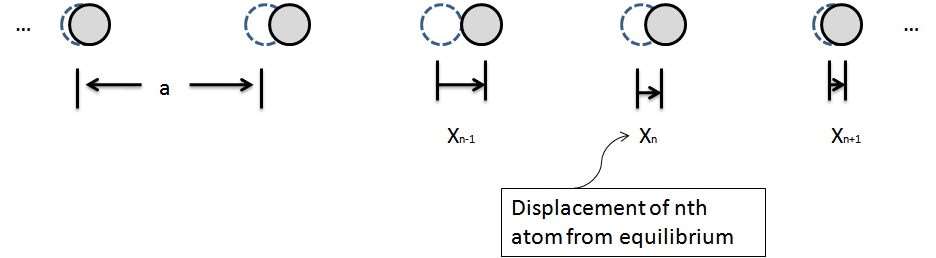
- Again, let us focus only on the possible normal modes for the system. Assuming that the positioning of the particles satisfies a normal mode, the envelope function of the particles will give the initial conditions. Define the envelope function for the $n$th particle as
$$x_{n}=\sin{kna} \; \; $$
where $na$ is the location of the nth atom and $k$ is the wave vector of the envelope function. The position function can be generalized by writing it as
$$x_{n}=Re\left[Ae^{ikna}\right] \, \, at \, \, t=0 \; \; .$$
- Let us add the time dependence for the position of the $n$th particle now as well.
$$when \; t>0,$$
$$x_{n}(t) \, = \, Re\left[Ae^{ikna}e^{i\omega_{k} t}\right] \; \; , $$
where $\omega_{k}$ is the frequency of the normal mode associated with this particular envelope function.
Similarly, the position function for the neighboring particles can be written as
$$x_{n+1}(t) \, = \, Re\left[Ae^{ik(n+1)a}e^{i\omega_{k} t}\right] \; \; $$
and
$$x_{n-1}(t) \, = \, Re\left[Ae^{ik(n-1)a}e^{i\omega_{k} t} \right] \; \; . $$
- Now, all we need to define the motion of the $n$th particle is the frequency of oscillation $\omega_{k}$. In all of our previous cases, information about the frequency has been found in the equations of motion derived from the forces on a particle. Let us see what we can find with this strategy; the equation of motion for the $n$th particle is written as
$$m\ddot{x}_{n} \, = \, -\kappa\left(x_{n}-x_{n-1}\right) - \kappa \left(x_{n}-x_{n+1}\right) \; \; .$$
- Let us plug in the expressions for $x_{n}$, $x_{n+1}$, and $x_{n-1}$ into the equation of motion and simplify what we can.
$$-m\omega_{k}^{2}e^{ikna} \, = \, -\kappa\left(e^{ikna}-e^{ik(n-1)a}\right) - \kappa \left(e^{ikna}-e^{ik(n+1)a}\right) \; \; .$$
Factoring out a term of $e^{ikna}$ will then give
$$m\omega_{k}^{2}=\kappa\left(1-e^{-ika}\right) + \kappa\left(1-e^{ika}\right) \; \; ,$$
$$m\omega_{k}^{2}=2\kappa -\kappa\left(e^{ika}+e^{-ika}\right) \; \; ,$$
$$m\omega_{k}^{2}=2\kappa\left(1- \cos{ka}\right) \; \; , $$
$$m\omega_{k}^{2}=2\kappa\left(2 \: \sin{^{2}\frac{ka}{2}}\right) \; \; , $$
$$\omega_{k}(k)=\left|\sqrt{\frac{4\kappa}{m}}\; \sin{\frac{ka}{2}}\right| \; \; . $$
- We have found the normal mode frequency as a function of the envelope function's wave vector. Let's plot the dispersion relation and see what we can learn about how a 1-d infinite chain behaves.
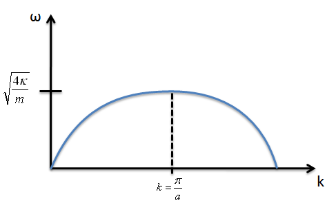
- Ask the class about any interesting characteristics of the dispersion relation they see.
Some important observations:
- There is a maximum frequency at which atoms in a solid can vibrate (This has profound implications for the heat capacity of solids).
- The velocity of sound waves, which have small wave vectors (long wavelength), can be predicted from
$$\omega \approx v_{sound}\, k $$
for small $k$.
- There are not any new normal modes described by $k > \frac{\pi}{a}$. All information for the oscillating system is contained in the range $k < \frac{\pi}{a}$. This region is called the first Brillouin Zone.