Table of Contents
Chapter 9: The Geometry of the Dot and Cross Products
A slightly expanded version of this chapter appears in [ 7 ].
9.1: Dot Product
Most students first learn the algebraic formula for the dot product in rectangular coordinates, and only then are shown the geometric interpretation. We believe it should be done in the other order. Students tend to remember best the first definition they use; this should not be an algebraic formula devoid of context. The geometric definition is coordinate independent, and therefore conveys invariant properties of the dot product, not just a formula for calculating it.
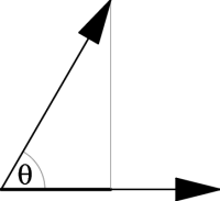 Figure 9.1: The dot product is fundamentally a projection.
The dot product is fundamentally a projection, as shown in Figure 9.1, which leads to the geometric formula \begin{equation} \vv\cdot\ww = {|\vv| |\ww| \cos\theta} \label{dotgeom} \end{equation} for the dot product of $\vv$ and $\ww$.
An immediate consequence of ($\ref{dotgeom}$) is that the dot product of a vector with itself gives the square of the length, that is \begin{equation} \vv\cdot\vv = |\vv|^2 \end{equation} In particular, taking the “square” of any unit vector yields 1, for example \begin{equation} \ii\cdot\ii = 1 \end{equation} Furthermore, it follows immediately from the geometric definition that two vectors are orthogonal if and only if their dot product vanishes, that is \begin{equation} \vv\perp\ww \Longleftrightarrow \vv\cdot\ww = 0 \end{equation}
If you use orthonormal basis vectors, such as $\{\ii,\jj,\kk\}$ for rectangular coordinates, then the geometric formula reduces to the standard component form of the dot product. For example, if $\vv=v_x\,\ii+v_y\,\jj$ and $\ww=w_x\,\ii+w_y\,\jj$, then 1) \begin{eqnarray} \vv\cdot\ww &=& (v_x\,\ii+v_y\,\jj)\cdot(w_x\,\ii+w_y\,\jj) \nonumber\\ &=& v_x w_x \,\ii\cdot\ii + v_y w_y \,\jj\cdot\jj + v_x w_y \,\ii\cdot\jj + v_y w_x \,\jj\cdot\ii \\ &=& v_x w_x + v_y w_y \nonumber \end{eqnarray} This computation clearly works for any orthonormal basis.
A special case is the dot product of a vector with itself, which reduces to the Pythagorean theorem, for example \begin{equation} \vv\cdot\vv = |\vv|^2 = v_x^2 + v_y^2 \end{equation}
 Figure 9.2: The Law of Cosines is just the definition of the dot product.
What happens if you don't use an orthonormal basis? Consider Figure 9.2, in which $\CC=\BB-\AA$. Then \begin{eqnarray} \CC\cdot\CC &=& (-\AA + \BB) \cdot (-\AA + \BB) \nonumber\\ &=& \AA\cdot\AA + \BB\cdot\BB - 2 \,\AA\cdot\BB \end{eqnarray} or equivalently \begin{equation} |\CC|^2 = |\AA|^2 + |\BB|^2 - 2|\AA||\BB|\cos\theta \end{equation} which is just the Law of Cosines.
A good problem which emphasizes both the geometric and algebraic representations of the dot product is to find the angle between the diagonal of a cube and one of its edges.
9.2: Gram-Schmidt orthogonalization
As discussed in §9.1 in Chapter 9, the component of a vector $\vv$ along a unit vector is simply the dot product of the two vectors, and if the vector projection is desired, it points in the direction of the unit vector. To project $\vv$ along a vector $\ww$ which isn't a unit vector, one constructs the unit vector $\ww\over|\ww|$ in the direction of $\ww$, and proceeds as before. Thus, the (scalar) component of $\vv$ in the direction of $\ww$ is \begin{equation} \hbox{component of $\vv$ along $\ww$} = \vv\cdot{\ww\over|\ww|} \end{equation} as shown in Figure 9.1. The (vector) projection of $\vv$ along $\ww$ is this component times the unit vector in the direction of $\ww$, namely \begin{equation} \hbox{projection of $\vv$ along $\ww$} = \left(\vv\cdot{\ww\over|\ww|}\right) \> {\ww\over|\ww|} = {\vv\cdot\ww\over\ww\cdot\ww} \> \ww \label{Projection} \end{equation}
Perhaps the most important application of the dot product is the use of ($\ref{Projection}$) to decompose vectors into their components parallel and perpendicular to a given vector. The Gram-Schmidt orthogonalization process uses this to construct an orthonormal basis from a given set of (linearly independent) vectors. This can be beautifully illustrated in three dimensions, as follows. Stick out three fingers of one hand in arbitrary directions. Pick one of these vectors, then a second, and subtract from the second its projection parallel to the first, resulting in a vector perpendicular to the first. Now subtract from the remaining vector its projections parallel to both the first and second vectors, resulting in a vector perpendicular to both. These three vectors can be normalized if desired, yielding an orthonormal basis.
9.3: Cross Product
We strongly discourage teaching, or even reviewing, the dot and cross products at the same time — students tend to get them mixed up! The dot product is needed right away, in order to discuss line integrals, whereas the cross product isn't really needed until one discusses surface integrals. 1)
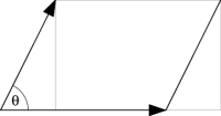 Figure 9.3: The geometric definition of the cross product.
The cross product is fundamentally a directed area. The magnitude of the cross product is defined to be the area of the parallelogram, as shown in Figure 9.3. This leads to the formula \begin{equation} |\vv\times\ww| = |\vv||\ww|\sin\theta \label{crossgeom} \end{equation} an immediate consequence of which is that \begin{equation} \vv\parallel\ww \Longleftrightarrow \vv\times\ww=\zero \label{Cross1} \end{equation} The direction of the cross product is given by the right-hand rule, so that in the example shown $\vv\times\ww$ points out of the page. This implies that \begin{equation} \vv\times\ww = - \ww\times\vv \label{Cross2} \end{equation} so that the cross product is not commutative. 2) An important property of the cross product is that \begin{equation} \vv\times\vv = \zero \end{equation} which follows from either ($\ref{Cross1}$) or ($\ref{Cross2}$).
In terms of the standard orthonormal basis, the geometric formula quickly yields \begin{eqnarray} \ii\times\jj &=& \kk \nonumber\\ \jj\times\kk &=& \ii \\ \kk\times\ii &=& \jj \nonumber \end{eqnarray} This cyclic nature of the cross product can be emphasized by abbreviating this multiplication table as shown in Figure 9.4. 3) Products in the direction of the arrow get a plus sign; products against the arrow get a minus sign.
 Figure 9.4: The cross product multiplication table.
Using an orthonormal basis such as $\{\ii,\jj,\kk\}$, the geometric formula reduces to the standard component form of the cross product. If $\vv=v_x\,\ii+v_y\,\jj+v_z\,\kk$ and and $\ww=w_x\,\ii+w_y\,\jj+w_z\,\kk$, then 4) \begin{eqnarray} \label{CrossAlg} \vv\times\ww &=& (v_x\,\ii+v_y\,\jj+v_z\,\kk) \times (w_x\,\ii+w_y\,\jj+w_z\,\kk) \\ &=& (v_y w_z - v_z w_y)\,\ii + (v_z w_x - v_x w_z) \,\jj + (v_x w_y - v_y w_x)\,\kk \end{eqnarray} which is often written as the symbolic determinant \begin{equation} \vv\times\ww = \left| \matrix{\ii& \jj& \kk\cr v_x& v_y& v_z\cr w_x& w_y& w_z\cr} \right| \label{CrossDet} \end{equation}
We emphasize that this works in any (right-handed) orthonormal basis. In cylindrical coordinates, not only is \begin{equation} \rhat\times\phat = \zhat \end{equation} but cross products can be computed as \begin{equation} \vv\times\ww = \left| \matrix{\rhat& \phat& \zhat\cr v_r& v_\phi& v_z\cr w_r& w_\phi& w_z\cr} \right| \end{equation} where of course $\vv=v_r\,\rhat+v_\phi\,\phat+v_z\,\zhat$ and similarly for $\ww$.
We strongly discourage students from memorizing ($\ref{CrossAlg}$), recommending ($\ref{CrossDet}$) instead. But we discourage students from working out the determinant using minors, which would result in the final expression in ($\ref{CrossAlg}$) but with 2 sign changes in the term involving $\jj$. Instead, we encourage students to take $3\times3$ determinants in the form  \begin{eqnarray} \end{eqnarray} where one multiplies the terms along each diagonal line, subtracting the products obtained along lines going down to the left from those along lines going down to the right. While this method works only for ($2\times2$ and) $3\times3$ determinants, and is therefore usually omitted from a linear algebra course, it has the definite advantage of emphasizing the cyclic nature of the cross product — whereas students who use minors often make sign errors.
More important than which method students use to compute determinants is encouraging them not to use determinants at all for simple cross products, such as $(\ii+3\,\jj)\times\kk$, but instead to use the multiplication table directly. It is also worth pointing out that the multiplication table and the determinant method generalize naturally to other orthonormal bases; all that is needed is to replace the rectangular basis $\{\ii,\jj,\kk\}$ by the one being used.
A good problem which emphasizes the geometry of the cross product is to find the area of the triangle formed by connecting the tips of the vectors $\ii$, $\jj$, $\kk$ (whose base is at the origin).
1)
We use the Murder Mystery Method, described in
Chapter 12,
rather than the cross product, to determine whether vector fields are
conservative.
2)
The cross product also fails to be associative, since for example
$\ii\times(\ii\times\jj)=-\jj$ but $(\ii\times\ii)\times\jj=\zero$.
3)
This is really the multiplication table for the unit imaginary
quaternions, a number system which generalizes the familiar complex numbers.
Quaternions predate vector analysis, which borrowed the $i$, $j$, $k$ notation
for the rectangular basis vectors $\ii$, $\jj$, $\kk$. A more logical name
would be $\xhat$, $\yhat$, $\zhat$, which is used by many physicists.