It is time to distinguish between several different vector-like objects. The arrow pointing from the origin to the point with (Cartesian) coordinates $(a,b,c)$ is $$\ww = a\,\ii + b\,\jj + c\,\kk$$ This is a vector, which is said to have its tail at the origin, or to live at the origin. There is nothing special about the origin; vectors can live at any point.

A vector function (of one variable) $$\ww(u) = f(u)\,\ii + g(u)\,\jj + h(u)\,\kk$$ is a vector for each value $u=u_0$ of its argument. One example is a parametric curve $\rr(u)$. We often identify the position vector $\rr=x\,\ii+y\,\jj+z\,\kk$ with the point $(x,y,z)$, and similarly for the corresponding vector function $\rr(u)$. For example, we sometimes write $f(\rr)$ rather than $f(x,y,z)$. A parametric curve is a special vector function, in that it always lives at the origin. Many vector functions live instead on a parametric curve, such as the velocity $\vv(u)$, which, for each value of $u$, lives at the point $\rr(u)$ on the curve.

Finally, a vector field $$\FF(x,y,z) = F_x(x,y,z)\,\ii + F_y(x,y,z)\,\jj + F_z(x,y,z)\,\kk$$ assigns a vector $\FF(x_0,y_0,z_0)$ to each point $(x_0,y_0,z_0)$, which lives at $(x_0,y_0,z_0)$. \footnote[1]{In two dimensions, of course, $F_z=0$, and $F_x=F_x(x,y)$, $F_y=F_y(x,y)$.} An example of a vector field is the gradient of a function, $\grad{f}$. It is common practice to omit the explicit functional dependence, and write simply $$\FF = F_x\,\ii + F_y\,\jj + F_z\,\kk$$ as it is usually clear from the context what type of object $\FF$ is. But be careful; the vector $\ii$ (a single arrow at the origin) is different from the constant vector field $\ii$ (an arrow at each point, all pointing in the $x$-direction).

In some settings, other bases are more appropriate. We have already introduced $\rhat$ and $\phat$, the unit vectors pointing in the directions of increasing $r$ and $\phi$, respectively. These are vector fields! If desired, one can work out explicit formulas for these vector fields in terms of $\ii$ and $\jj$, but these are not needed to draw pictures of these vector fields, which are shown below.

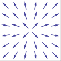
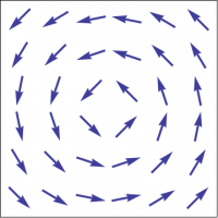
It is obvious geometrically that $$\rhat \cdot \phat = 0$$ at every point, so that $\{\rhat,\phat\}$ is an orthonormal basis for vector fields in the plane. 1) We can thus expand a vector field $\FF$ in the plane with respect to either basis, yielding \begin{eqnarray*} \FF &=& F_x \,\ii + F_y \,\jj \\ &=& F_r \,\rhat + F_\theta \,\phat \end{eqnarray*} where $F_r$ denotes the $r$-component of $\FF$, etc. Similar expressions hold for cylindrical and spherical coordinates.

Most mathematics textbooks always use the Cartesian (also called rectangular) basis $\{\ii,\jj,\kk\}$, which has the advantage of establishing a single formalism for all situations. But problems involving special symmetry, such as cylindrical or spherical symmetry, are usually much simpler if the computation is done in an adapted basis, such as those appropriate for cylindrical and spherical coordinates. Remarkably, essentially all of undergraduate engineering and physics can be handled by mastering these special cases! For this reason, engineering and physics texts typically emphasize the use of an adapted basis.

The bottom line is that all problems in this course can be solved using only rectangular basis vectors, but that many problems, both now and in your future coursework, are likely to be much easier if you learn how to work with other basis vectors. Ideally, you should learn both approaches, and know how they are related.

GOALS