Table of Contents
Chapter 3: The Vector Differential
3.1: Small Changes in Position
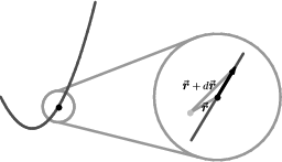 Figure 3.1: The infinitesimal displacement vector $d\rr$ along a curve, shown in an
“infinite magnifying glass”. In this and subsequent figures, artistic
license has been taken in the overall scale and the location of the origin
in order to make a pedagogical point.
Figure 3.1: The infinitesimal displacement vector $d\rr$ along a curve, shown in an
“infinite magnifying glass”. In this and subsequent figures, artistic
license has been taken in the overall scale and the location of the origin
in order to make a pedagogical point.
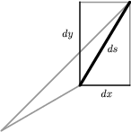
Figure 3.2a:
The infinitesimal version of the Pythagorean Theorem.
The position vector 1) \begin{equation} \rr=x\,\ii+y\,\jj+z\,\kk \end{equation} describes the location of the point $(x,y,z)$ in rectangular coordinates. It is instructive to draw a picture of the small change $\Delta\rr=\Delta x\,\ii + \Delta y\,\jj + \Delta z\,\kk$ in the position vector between nearby points. Try it! This picture is so useful that we will go one step further, and consider an infinitesimal change in position. Instead of $\Delta\rr$, we will write $d\rr$ for the vector between two points which are infinitesimally close together. This is illustrated in Figure 3.1, which shows a view of the curve through an “infinite magnifying glass”.
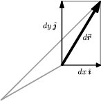
Figure 3.2b:
The vector version of the Pythagorean Theorem in rectangular
coordinates.
Note that, like any vector, $d\rr$ can be expanded with respect to $\ii$, $\jj$, $\kk$; the components of $d\rr$ are just the infinitesimal changes $dx$, $dy$, $dz$, in the $x$, $y$, and $z$ directions, respectively, that is \begin{equation} d\rr = dx\,\ii + dy\,\jj + dz\,\kk \label{drdef} \end{equation} You may find this intuitive notion of $d\rr$ as an infinitesimal vector displacement to be helpful in visualizing the geometry of vector calculus.
What is the infinitesimal distance $ds$ between nearby points? Just the length of $d\rr$! We have \begin{equation} ds = |d\rr| \label{dsdef} \end{equation} and squaring both sides leads to \begin{equation} ds^2 = |d\rr|^2 = d\rr\cdot d\rr = dx^2 + dy^2 + dz^2 \label{ds1} \end{equation} which is just the infinitesimal Pythagorean Theorem, as shown in Figure 3.2. 2)
3.2: Other Coordinate Systems
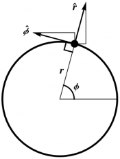
It is important to realize that $d\rr$ and $ds$ are defined geometrically, not by ($\ref{drdef}$) and ($\ref{dsdef}$). To emphasize this coordinate-independent nature of $d\rr$, it is useful to study $d\rr$ in another coordinate system, such as polar coordinates ($r$,$\phi$) in the plane. 1) It is also natural to introduce basis vectors $\{\rhat,\phat\}$ adapted to these coordinates, with $\rhat$ being the unit vector in the radial direction, and $\phat$ being the unit vector in the direction of increasing $\phi$. One can of course relate $\rhat$ and $\phat$ to $\ii$ and $\jj$, for instance using the first drawing in Figure 3.3. However, in most physical applications (as opposed to problems in calculus textbooks) this can be avoided by making an appropriate initial choice of coordinates.
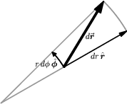
Figure 3.2c:
The infinitesimal vector version of the Pythagorean Theorem,
in polar coordinates.
Determining the lengths of the sides of the resulting infinitesimal polar “rectangle”, one obtains \begin{equation} d\rr = dr\,\rhat + r\,d\phi\,\phat \label{dr2} \end{equation} as shown in Figure 3.2c. Using ($\ref{dsdef}$) and squaring both sides as before leads to \begin{equation} ds^2 = dr^2 + r^2 \, d\phi^2 \label{ds2} \end{equation} which is the infinitesimal Pythagorean Theorem in polar coordinates
Analogous expressions can be derived for $d\rr$ in other coordinate systems, some of which we will use below. A worksheet which we often assign for homework is attached at the end of this chapter.
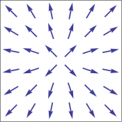
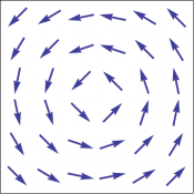
When using basis vectors adapted to curvilinear coordinates, it is essential to realize that the basis vectors are not constant. The polar basis $\{\rhat,\phat\}$ is shown in Figure 3.3.
3.3: Vector Differentials
Vector derivatives are now easy. The vector differential $d\rr$ along a curve is the vector between points (along the curve) which are infinitesimally close. But what does this mean? “Infinitesimal” simply means to zoom in on the curve so much that it becomes straight.
Parametric curves can be described by viewing the position vector $\rr$, and hence also $x$, $y$, and $z$ as functions of some parameter $u$. “Dividing” the expression for $d\rr$ in ($\ref{drdef}$) by $du$ leads to the derivative \begin{equation} {d\rr\over du} = {dx\over du}\,\ii + {dy\over du}\,\jj + {dz\over du}\,\kk \end{equation} You may view this as a purely formal manipulation, although it is often used as the definition of the vector differential $d\rr$, that is \begin{equation} d\rr = {d\rr\over du} \,du \label{olddef} \end{equation} You may also wish to compare this with the traditional definition of the derivative of the position vector, namely \begin{equation} {d\rr\over du} = \lim_{\Delta u\to0} {\Delta\rr\over\Delta u} \end{equation} which again illustrates that derivatives are ratios of infinitesimal changes.
We choose to work directly with differentials. The fundamental relations are the above expressions for $d\rr$, namely ($\ref{drdef}$) in rectangular coordinates, and ($\ref{dr2}$) in polar coordinates. Similar expressions hold in other coordinates.
3.4: Calculating Line Elements
Below is a link to a worksheet students can use to construct the vector differential $d\rr$ in both cylindrical and spherical coordinates. We have used this worksheet successfully both as an in-class activity and for homework.