The index of a vector field at a point on a 2-dimensional surface is a measure of how many times the vector field "rotates" about that point. Imagine drawing a small circle about the point, and keeping track of the angle between the vector field and the circle as you go around the circle. The result must be a multiple of $2\pi$; the multiplicity is the index. Thus, if a smooth vector field is nonzero in a neighborhood, its index is $0$ at every point in the neighborhood. The Poincaré–Hopf Theorem states that a vector field $\vv$ on a compact surface $M$ satisfies $$\chi(M) = \sum\ind(\vv,p)$$ where $\chi$ denotes the Euler characteristic, $\ind(\vv,p)$ the index of $\vv$ at $p\in M$, and the sum is over the isolated singularities of $\vv$, that is, the points $p$ where $\vv$ is either zero or undefined.
The images below show spherical vector fields with particular index structures. Since the Euler characteristic of the sphere is $2$, the total index must be $2$ in each case. The first two figures show vector fields with two singular points of index $1$; the first example has an obvious source and sink, whereas the second has neither. These two examples are just the coordinate basis vector fields $\ee_1=\partial_\theta$ and $\ee_2=\partial_\phi$, respectively, where $\theta$ denotes colatitude, and $\phi$ denotes longitude.


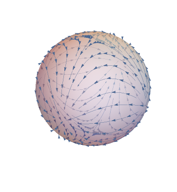
The next figure shows a vector field with a single singular point of index $2$, obtained by mapping the singularity-free vector field $\xhat=\partial_x$ in the plane to the sphere using stereographic projection.

Finally, the last figure shows a vector field with six singular points, four of index $1$, and two of index $-1$. The former are arranged as alternating sources and sinks around the equator, and the latter are at the poles. This vector field was constructed from the electric field of a quadrupole, with four charges of equal magnitude but alternating signs on the equator; the resulting vector field vanishes at the poles.