ANNOUNCEMENTS
MTH 255 - Winter 2001

All chapter numbers are based on the Early Transcendentals version of the 4th edition of the text,
and must be increased by one for the Multivariable version.
For further information, click here.

3/26/01

Below are the answers to the final; an answer key is available in my office.

1. (a) false (b) true

2. (a) div (F) > 0 (b) curl (F) · k < 0

3. (a) conservative; g=x+xy+xyz+z² (b) not conservative

4. 2

5. (a) (2i+2j+k)/3 (b) 4

6. 81 Pi

7. -256 Pi

8. (a) 2 Pi (b) 0 (EC) 2 Pi

See me to pick up your final exam and/or to double-check your grade.

3/21/01

An incorrect answer to Problem 1c on the sample final is given in the solutions; the correct answer is 1.

A sample change of variables problem is:

Compute the double integral of sin(2x+y) dA over the region D bounded by the lines -x+4y=4, -x+4y=12, 2x+y=4, 2x+y=Pi.

(This was Problem 5 on the sample exam for the second midterm; the answer can be found here.)

3/16/01

Office hours during finals week: Johnner: MT 3-4 PM; Tevian: WR 9-11:30 AM (roughly)

Review session: 3-4:30 PM on Wednesday 3/21 in Kidd 280.

3/14/01 (Einstein's birthday!)

Here's the review problem mentioned in class: Find the flux of the vector field F = (x²+y²+z²) (x i+y j+z k) outwards through the closed cylinder x²+y²=4, whose ends are given by z=0 and z=3.

You should be able to solve this problem in 2 different ways; the correct answer is 300 Pi.

3/12/01

The final is 6-7:50 PM on Thursday 3/22 in Kidd 364 (our regular classroom):

Roughly 50% of the final will cover new material.

The remaining 50% of the final will consist of questions which could have been on one of the midterms.

The new material consists of Lessons 11-15 in the Study Guide (§15.9 & §16.6-§16.9 in the text).

    (3-d change of variables will not be tested.)

There is also a very nice summary of the main theorems in §16.10.

You should study the review sections at the end of Chapters 11, 12, 13, and 14.

The exam is closed book, and calculators may not be used.

You may bring three 3×5 index cards (both sides) OR one 8½×11 piece of paper (one side) of handwritten notes.

Friday's lecture will be devoted to review. Come prepared to ask questions!

3/9/01

The formulas shown in class today for the divergence and curl in spherical and cylindrical coordinates are from the inside front cover of the widely used physics textbook entitled Introduction to Electrodynamics by David Griffiths. The derivation of these formulas is briefly discussed in an appendix of that book; an expanded discussion can be found in the excellent book div, grad, curl and all that, by H M Schey. Both books are available in the library.

3/7/01

You can find a sample final (not written by me) here.

(The solutions are here, but please try the problems without peeking first.)

3/5/01

A Java-based "microscope" for visualizing vector fields can be found here.

This tool allows one to see the divergence and curl directly; try it!

2/23/01

Today is the last day to withdraw! Please see me if you would like to discuss how you are doing in the class.

2/21/01

Below are the answers to the second midterm; an answer key has been posted outside my office.

1. (a) not conservative (b) conservative; f=x³+yz²+xe^ysinz

2. (a) 0 (b) 1

3. -9 Pi

4. (a) conservative (b) not conservative (c) conservative (d) not conservative

5. 16/3+4 Pi

2/15/01

The following material in §14.5 will not be on the midterm:

The divergence of a vector field; vector forms of Green's Theorem; flux.

Problems 2(b) and 4(b) on the sample midterm deal with these topics; you do not (yet) need to know how to solve these problems (nor Problem 5).

2/13/01

The second midterm is in class on Monday 2/19:

The midterm covers Lessons 6-10 in the Study Guide (§16.1-§16.5 in the text).
(We will not cover the divergence of a vector field until after the exam.)

You should also study the review section at the end of Chapter 16.

You can find a sample midterm (not written by me) here.

The exam is closed book, and calculators may not be used.

You may bring two 3×5 index cards (both sides) of handwritten notes;

Here are the double angle formulas you may need for the exam:
   sin(2t)=2sin(t)cos(t); cos(2t)=cos²t-sin²t   so that   cos²t=(1+cos(2t))/2; sin²t=(1-cos(2t))/2;

Friday's lecture will be devoted to review. Come prepared to ask questions!

2/12/01

Example 2 in §16.4 is a good example of the use of Green's Theorem, since both difficult terms vanish when differentiated. While polar coordinates do indeed simplify the integral, there's no need to bother, since the integral is just 4 times the area of the circle of radius 3 -- which the book doesn't mention!

2/5/01

Here are the figures constructed by Maple during the computer demo shown in class today. The surface shown is the graph of the function f(x,y)=2*x*sin(Pi*y). The remaining figures depict the line integral of this function along different paths (shown in blue) from (0,0) to (1,1). In each case, the result of the integration gives the area between the red and blue curves. Path 1 is a straight line, Path 2 consists of 2 line segments parallel to the axes, and Path 3 is a curve. (The red curves do not show up well in this format.)

1/31/01

Below are the answers to the first midterm; an answer key has been posted outside my office.

1. a_T=1; a_N=2; K=2/9

2. min at (0,-4); saddle at (2,-4)

3. absolute min of 0 at (2,2); absolute max of 16 at (-2,-2)

4. 4/5 i+3/5 j

5. -1/300 °C/m (decreases)

1/29/01

A missing factor of 2 has been added to the answer to Problem 3b on the list of review problems.

1/28/01

Here are the answers to the review problems:

1. r = (2t-sin(t)) i+(2t-cos(t)+1) j+(2e^t-t-2) k     (v = dr/dt)

2. (a) v = 3e^t i+(2t+4) j ; a = 3e^t i+2t j (b) v = 3 i+4 j ; v = 5 ; a = 3 i+2 j

    (c) T = 3/5 i+4/5 j ; N = 4/5 i-3/5 j ; K = 6/125 ; a_T = 17/5 ; a_N = 6/5

3. (a) 5 (b) (8 i+9 j+2 k)/149^1/2 ; 149^1/2/2 (c) 8x+9y+2z = 25

4. saddle at (0,0); min at (1,1)

5. min=1-30^1/2 at (-3/5,-2/5)*30^1/2 ; max=1+30^1/2 at (3/5,2/5)*30^1/2

1/26/01

You are not responsible for the method of Lagrange multipliers with 2 constraints. But you should know how to use the method of Lagrange multipliers in 2 dimensions, that is, for functions of 2 variables. The main use of this method, at least in this course, will be to find the min/max of a function along the boundary of a region.

The first 3 figures in §14.8 show the geometry behind the method of Lagrange multipliers.

Here's the example from the end of today's lecture:

Find the points on the curve x²+xy+y²=3 whose distance from the origin is a maximum or a minimum.

It is instructive to try this problem both by setting grad f = lambda (grad g) (the method in the text) and by setting grad f × grad g = 0 (the method described in class). The first method leads to an eigenvalue problem with 2 separate cases to consider; the second is much more straightforward.

1/25/01

You can use Maple to graph equations! In 2d, you can use the command "implicitplot", for example:

with(plots):
implicitplot(x^2+y^2=25,x=-5..5,y=-5..5,scaling=constrained);

but in 3d you must use "implicitplot3d", for example:

with(plots):
implicitplot3d(x^2+y^2+z=50,x=-5..5,y=-5..5,z=25..50);

1/24/01

The first midterm is in class on Wednesday 1/31:

The midterm covers Lessons 1-5 in the Study Guide (§13.1-§13.4 and §14.6-14.8 in the text).

You should also study the review sections at the end of Chapters 13 and 14.

You can find some review questions (not written by me) here.

The exam is closed book, and calculators may not be used.

You may bring a 3×5 index card (both sides) of handwritten notes;

Bring your OSU ID to the exam!

Monday's lecture will be devoted to review. Come prepared to ask questions!

1/22/01
Here is an example of a function of 2 variables with 2 local maxima but no local minima -- something which is not possible for (continuous) functions of 1 variable.
(The graph shown is z = - (x²-1)² - (yx²-x-1)².)

1/19/01

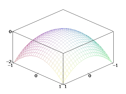
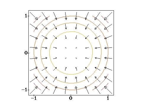
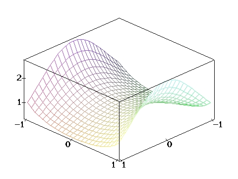
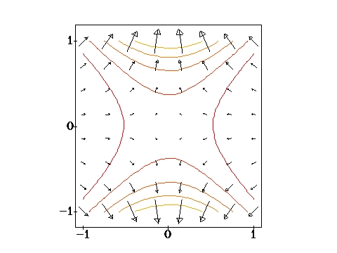
Here are the figures shown in class today, drawn using Maple. In each case, the first picture shows the (3-d!) graph of a function z = f(x,y), and the second shows the combined (2-d!) graph of the level curves and gradient of f.

1/18/01

Lab 2 turned out to be too long; you only need to write up the first 2 questions.

Some further information about differentials can be found in §14.4. You may wish to try problems §14.4: 23, 25.

1/12/01

Lab writeups are due at the end of Johnner's office hour (3-4 PM) on Friday. They can also be turned in during lecture, or during my office hour from 1-2 PM.

1/11/01

BOTH recitation rooms have been changed (and in one case changed back again)!
Check the course home page for the new rooms!

1/10/01

You can use Maple to graph parametric curves. For 2d curves, you can use the command "plot", for example:

plot([cos(t),sin(t),t=0..2*Pi]);

but for 3d parametric curves you must use "spacecurve", for example:

with(plots):
spacecurve([t,t^2,t^3],t=0..1);

Note that the syntax of these 2 commands is different!

(A Student Edition of Maple is available.)

1/9/01

My regular office hours are MWF at 1 PM, which is immediately after class. If nobody is waiting for me after 1:30 or so, I may leave, so if you're planning on coming after that, try to let me know beforehand, for instance by telling me at the end of class.

I am also usually in my office TW mornings, which are good times to make an appointment. Feel free to drop in at these times, but if you want to make sure I'm available, email me (tevian@math.orst.edu) or call me (737-5159) first. (I respond to email almost immediately if I'm in my office.)

1/8/01

The review material on vectors mentioned in class today can be found in §12.2-§12.5.

You may wish to try the following problems: §12.3: 11, 57; §12.4: 25; §12.5: 27.

You should also review the chain rule (§14.5) and multiple integration, especially double integrals (§15.3-§15.4).

A copy of the Early Transcendentals version of the 4th edition of the textbook is on reserve at the library.

1/5/01

Make sure to read the note about the various editions of the text.

The current version of the Study Guide is dated 7 December 2000. Earlier versions can be used, but please note that in this case all section numbers (and suggested problems) refer to the 3rd edition of Stewart. The suggested problems for the 4th edition can be found here.

Make sure to read the grading policy.