ANNOUNCEMENTS
MTH 255 - Spring 2001

All chapter numbers are based on the Early Transcendentals version of the 4th edition of the text,
and must be increased by one for the Multivariable version.
For further information, click here.

6/12/01

Below are the answers to the final; I'll post an answer key outside my office as soon as I can.

1. 3/25

2. (a) conservative; g=x+xy+xyz+z² (b) not conservative

3. (a) Figure 3; (b) Figure 1; (c) Figure 2;

4. 135/4

5. (a) (2i+2j+k)/3 (b) 8/3

6. 81 Pi/2

7. -32 Pi/3

8. (a) 2 Pi (b) 0

Exams will probably not be graded until Friday; grades will probably not be available until Monday. You can try catching me on either of those days to pick up your final.

6/8/01

I will give a brief lecture about relativity at 7 PM on Tuesday, 6/12, in Kidd 350 (our regular classroom). This talk is aimed at students in MTH 255; no further knowledge of math or physics will be assumed.

6/7/01

Here's the review problem mentioned yesterday in class: Find the flux of the vector field F = (x²+y²+z²) (x i+y j+z k) outwards through the closed cylinder x²+y²=4, whose ends are given by z=0 and z=3.

You should be able to solve this problem in 2 different ways; the correct answer is 300 Pi.

6/6/01

There will be a review session in Kidd 350 (our usual classroom) starting at 7 PM on Sunday, 6/10.

I will have extra office hours on Monday, 6/11, from approximately 3:15-4:30 PM.

Johnner will have extra office hours on Monday, 6/11, at 11 AM and again at 2 PM.

This week's lab will be due as usual in Johnner's office by 3 PM on Monday, 6/11.

6/5/01

The final is 9:30-11:20 AM on Tuesday 6/12 in Wngr 151.

Roughly 50% of the final will cover new material.

The remaining 50% of the final will consist of questions which could have been on one of the midterms.

The new material consists of Lessons 11-15 in the Study Guide (§15.9 & §16.6-§16.9 in the text).

    (3-d change of variables will not be tested.)

There is also a very nice summary of the main theorems in §16.10.

You should study the review sections at the end of Chapters 11, 12, 13, and 14.

The exam is closed book, and calculators may not be used.

You may bring three 3×5 index cards (both sides) OR one 8½×11 piece of paper (one side) of handwritten notes.

Friday's lecture will be devoted to review. Come prepared to ask questions!

6/4/01

You can find a sample final (not written by me) here.

(The solutions are here, but please try the problems without peeking first.)

6/1/01

The formulas shown in class today for the divergence and curl in spherical and cylindrical coordinates are from the inside front cover of the widely used physics textbook entitled Introduction to Electrodynamics by David Griffiths. The derivation of these formulas is briefly discussed in an appendix of that book; an expanded discussion can be found in the excellent book div, grad, curl and all that, by H M Schey. Both books are available in the library.

5/24/01

Today's lab is due in class on Wednesday, May 30.

5/15/01

Below are the answers to the second midterm; an answer key will be posted outside my office.

1. (a) not conservative (b) conservative; g=x³+yz²+x² sin(y) cos(z)

2. (a) conservative (b) not conservative (c) not conservative (d) conservative

3. -6

4. Pi²/8

5. 12 Pi

5/11/01

Matthias Kawski will give the Mathematics Department Colloquium on Tuesday, May 15, at 3 PM, in Kidder 364:

Technology in Vector Calculus -- zoom in to "see" the curl

A Java-based "microscope" for visualizing vector fields, designed by Professor Kawski, can be found here.

This tool allows one to see the divergence and curl directly; try it!

5/9/01

The second midterm is 12 PM on Monday 5/14 in Gilfillan Auditorium.

The midterm covers Lessons 6-10 in the Study Guide (§16.1-§16.5 in the text).

The following material in §14.5 will not be on the midterm: divergence; flux; 2-d divergence theorem.

You should also study the review section at the end of Chapter 16.

You can find a sample midterm (not written by me) here.

You do not (yet) need to know how to solve Problems 2(b) and 4(b) (nor Problem 5).

The exam is closed book, and calculators may not be used.

You may bring two 3×5 index cards (both sides) of handwritten notes;

Here are the double angle formulas you may need for the exam:
   sin(2t)=2sin(t)cos(t); cos(2t)=cos²t-sin²t   so that   cos²t=(1+cos(2t))/2; sin²t=(1-cos(2t))/2;

Friday's lecture will be devoted to review. Come prepared to ask questions!

5/7/01

Example 2 in §16.4 is a good example of the use of Green's Theorem, since both difficult terms vanish when differentiated. While polar coordinates do indeed simplify the integral, there's no need to bother, since the integral is just 4 times the area of the circle of radius 3 -- which the book doesn't mention!

5/3/01

There is a minor mistake in the wording of Problem 4b on Lab 5, which should say:

"... this integral is (mu₀ times) the current ..."

4/27/01

Here are the figures constructed by Maple during the computer demo shown in class today. The surface shown is the graph of the function f(x,y)=2*x*sin(Pi*y). The remaining figures depict the line integral of this function along different paths (shown in blue) from (0,0) to (1,1). In each case, the result of the integration gives the area between the red and blue curves. Path 1 is a straight line, Path 2 consists of 2 line segments parallel to the axes, and Path 3 is a curve. (The red curves do not show up well in this format.)

4/24/01

Yes, there is a lab this week. It should be shorter than usual, and there should be time left to go over the exam.

4/23/01

Below are the answers to the first midterm; an answer key will be posted outside my office.

1. (a) 4 (b) 0 (c) 0 (d) 2k

2. (a) saddle at (0,0) (b) min is -1, max is 1

3. (-3i+4j)/5

4. (a) (2i+j+2k)/3 (b) -1/500 °C/m (decreases)

5. a_T=0; a_N=4

4/20/01

Here are the answers to the review problems:

1. r = (2t-sin(t)) i+(2t-cos(t)+1) j+(2e^t-t-2) k     (v = dr/dt)

2. (a) v = 3e^t i+(2t+4) j ; a = 3e^t i+2t j (b) v = 3 i+4 j ; v = 5 ; a = 3 i+2 j

    (c) T = 3/5 i+4/5 j ; N = 4/5 i-3/5 j ; K = 6/125 ; a_T = 17/5 ; a_N = 6/5

3. (a) 5 (b) (8 i+9 j+2 k)/149^1/2 ; 149^1/2/2 (c) 8x+9y+2z = 25

4. saddle at (0,0); min at (1,1)

5. min=1-30^1/2 at (-3/5,-2/5)*30^1/2 ; max=1+30^1/2 at (3/5,2/5)*30^1/2

4/19/01

You can use Maple to graph equations! In 2d, you can use the command "implicitplot", for example:

with(plots):
implicitplot(x^2+y^2=25,x=-5..5,y=-5..5,scaling=constrained);

but in 3d you must use "implicitplot3d", for example:

with(plots):
implicitplot3d(x^2+y^2+z=50,x=-5..5,y=-5..5,z=25..50);

This is useful if you want to sketch the boundary of a region, but you only know the equation for the boundary in the form of a level curve, that is, with some function equal to a constant.

4/18/01

You are not responsible for the method of Lagrange multipliers with 2 constraints. But you should know how to use the method of Lagrange multipliers in 2 dimensions, that is, for functions of 2 variables. The main use of this method, at least in this course, will be to find the min/max of a function along the boundary of a region.

To find the max and min of the function f on the level curve g=const, find all points where grad f is parallel to grad g; those points are the only places where f might have a max or min on the given curve.

(To determine at which points f actually does have a min or max, make a table.)

The first 3 figures in §14.8 show the geometry behind the method of Lagrange multipliers.

Here's the example from the transparency in today's lecture:

Find the points on the curve x²+xy+y²=3 whose distance from the origin is a maximum or a minimum.

It is instructive to try this problem both by setting grad f = lambda (grad g) (the method in the text) and by setting grad f × grad g = 0 (the method described in class). The first method leads to an eigenvalue problem with 2 separate cases to consider; the second is much more straightforward.

4/17/01

The first midterm is 12 PM on Monday 4/23 in Gilfillan Auditorium.

The midterm covers Lessons 1-5 in the Study Guide (§13.1-§13.4 and §14.6-14.8 in the text).

You should also study the review sections at the end of Chapters 13 and 14.

You can find some review questions (not written by me) here.

The exam is closed book, and calculators may not be used.

You may bring a 3×5 index card (both sides) of handwritten notes;

Please write your exams in pencil or black ink (blue ink is OK).

Please turn off all electronic devices, such as cell phones and alarms; this also includes personal music players.

Friday's lecture will be devoted to review. Come prepared to ask questions!

A copy of the Early Transcendentals version of the 4th edition of the textbook is on reserve at the library.

4/16/01
Here is an example of a function of 2 variables with 2 local maxima but no local minima -- something which is not possible for (continuous) functions of 1 variable.
(The graph shown is z = - (x²-1)² - (yx²-x-1)².)

4/13/01

Strange but true: The 13th of the month is more likely to be a Friday than any other day of the week!

4/11/01

I may have announced the homework incorrectly in class on Monday.

The correct assignment can be found here.

Some further information about differentials can be found in §14.4. You may wish to try problems §14.4: 23, 25.

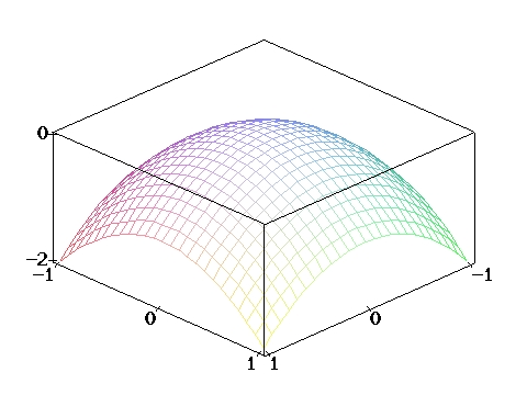
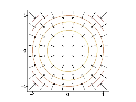
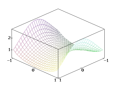
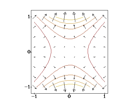
The figures shown in class today appear below, drawn using Maple. In each case, the first picture shows the (3-d!) graph of a function z = f(x,y), and the second shows the combined (2-d!) graph of the level curves and gradient of f.

As mentioned in class, Maple changes the overall scale of the arrows to get a nice picture..

4/10/01

You can use Maple to graph parametric curves. For 2d curves, you can use the command "plot", for example:

plot([cos(t),sin(t),t=0..2*Pi]);

but for 3d parametric curves you must use "spacecurve", for example:

with(plots):
spacecurve([t,t^2,t^3],t=0..1);

Note that the syntax of these 2 commands is different!

(A Student Edition of Maple is available.)

4/4/01

Office hours are now listed on the course homepage.

Lab writeups will be due each week at 3 PM on the Monday following the lab. They can be turned in during class, or during any of our Monday office hours.

This will also be true on midterm days! However, there will be no homework component to those labs.

4/3/01

The schedule for the first week has been changed slightly; some material from Lessons 1 & 2 will be presented both Wednesday and Friday.

4/2/01

The review material on vectors mentioned in class today can be found in §12.2-§12.5.

You may wish to try the following problems: §12.3: 1, 11, 57; §12.4: 9, 25; §12.5: 27.

The equation of the plane through the points (1,0,0), (0,1,0), (0,0,1) is x+y+z=1.

(This is the problem I didn't quite finish in class.)

You should also review the chain rule (§14.5) and multiple integration, especially double integrals (§15.3-§15.4), but also triple integrals (§15.7-§15.8).

3/30/01

Make sure to read the note about the various editions of the text.

The current version of the Study Guide is dated 7 December 2000. Earlier versions can be used, but please note that in this case all section numbers (and suggested problems) refer to the 3rd edition of Stewart. The suggested problems for the 4th edition can be found here.

Make sure to read the grading policy.

3/26/01

Students from last term should see me if they want to pick up their final exam and/or double-check their grade.