ANNOUNCEMENTS
MTH 255 - Fall 2000

12/7/00

Below are the answers to the final.

1. 4/25

2. 2x+2y-z=6

3. (a) NOT conservative; (b) conservative; g=x³+yz²+ xe^y sinz

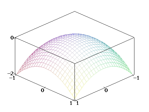
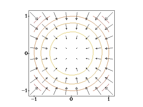
4. (a) Figure 3; (b) Figure 1; (c) Figure 2

    (div F>0 means radially outwards; (curl F) · k>0 means counterclockwise)

5. 2/3

6. -40 Pi (do the integral)

7. -32 Pi (Divergence Theorem)

8. (a) 2 Pi (do the integral); (b) 0 (Stokes' Theorem)

12/6/00

An answer key to the final has been posted outside my office. The exams will be graded by tomorrow morning, but grades won't be available until Friday. I will send you your grades via email provided you send me a request from an OSU email account in your own name.

11/29/00

Friday's lecture will be devoted to review. Come prepared to ask questions!

There will also be a review session in Kidd 350 (our regular classroom) on Monday 12/4 from 6-8 PM.

11/28/00

If you would like to check the raw data in my spreadsheet for your grades, please ask me.

If you are willing to be contacted later in the year for an anonymous survey regarding the effectiveness of this course, please give me your email address (which you can do by sending me an email message).

11/27/00

The final is 2-3:50 PM on Tuesday 12/5 in Kidd 350 (our regular classroom):

Roughly 50% of the final will cover new material.

The remaining 50% of the final will consist of questions which could have been on one of the midterms.

The new material consists of Lessons 11-15 in the Study Guide (§15.9 & §16.6-§16.9 in the text).

    (3-d change of variables will not be tested.)

There is also a very nice summary of the main theorems in §16.10.

You should study the review sections at the end of Chapters 11, 12, 13, and 14.

The exam is closed book, and calculators may not be used.

You may bring three 3×5 index cards (both sides) OR one 8½×11 piece of paper (one side) of handwritten notes.

11/22/00

You can find a sample final (not written by me) here.

(The solutions are here, but please try the problems without peeking first.)

11/20/00

A Java-based "microscope" for visualizing vector fields can be found here.

This tool allows one to see the divergence and curl directly; try it!

11/10/00

Today is the last day to withdraw! Please see me after class if you would like to discuss how you are doing in the class. If you want to see me after 2 PM, make sure I know about it before then, as I will otherwise leave at about that time.

11/8/00

Below are the answers to the second midterm; an answer key has been posted outside my office.

1. (a) 0 (b) 4 (c) 4

2. (a) conservative; g = xyz + xy + x + z² (b) not conservative

3. -9 Pi

4. (a) conservative (b) not conservative

5. Pi/2 + 2/3

11/3/00

Example 2 in §16.4 is a good example of the use of Green's Theorem, since both difficult terms vanish when differentiated. While polar coordinates do indeed simplify the integral, there's no need to bother, since the integral is just 4 times the area of the circle of radius 3 -- which the book doesn't mention!

10/30/00

The second midterm is in class on Monday 11/6:

The midterm covers Lessons 6-10 in the Study Guide (§16.1-§16.5 in the text).

You should also study the review section at the end of Chapter 16.

You can find a sample midterm (not written by me) here.

The exam is closed book, and calculators may not be used.

You may bring two 3×5 index cards (both sides) of handwritten notes;

Here are the double angle formulas you may need for the exam:
   sin(2t)=2sin(t)cos(t); cos(2t)=cos²t-sin²t   so that   cos²t=(1+cos(2t))/2; sin²t=(1-cos(2t))/2;

Friday's lecture will be devoted to review. Come prepared to ask questions!

10/29/00

Strange but true: Two people are talking on the telephone. Both are in the continental United States. One is in a state which borders the Atlantic Ocean; the other is in a state which borders the Pacific Ocean. They suddenly realize that the correct local time in both locations is the same! How is this possible?

10/27/00

Here's a good example of when to use the "long" version of the area corollary. Consider the graph of the equation x^2/3+y^2/3=1. (Try to graph this on your calculator or computer!) A parameterization is x=cos³t; y=sin³t, with t going from 0 to 2*Pi. Find the area inside using Green's Theorem. (The correct answer is 3*Pi/8.)

10/20/00

Here are the figures shown in class today. The surface shown is the graph of the function f(x,y)=2*x*sin(Pi*y). The remaining figures depict the line integral of this function along different paths (shown in blue) from (0,0) to (1,1). In each case, the result of the integration gives the area between the red and blue curves. Path 1 is a straight line, Path 2 consists of 2 line segments parallel to the axes, and Path 3 is a curve. (The red curves do not show up well in this format.)

10/16/00

Below are the answers to the first midterm; an answer key has been posted outside my office.

1. (a) 2/3 i+1/3 j+2/3 k (b) 0 (c) 2(x-1)+1(y-2)+2(z-3)=0 (or any multiple)

2. saddle at (0,0)

3. absolute min of -4 at (2,-2) and (-2,2) ; absolute max of 1 at (1,1) and (-1,-1)

4. T = 3/5 i+4/5 j ; N = -4/5 i+3/5 j ; K = 12/125

5. 0 (x+y=1 is a straight line!)

10/13/00

Strange but true: The 13th of the month is more likely to be a Friday than any other day of the week!

10/12/00

Answers to the review problems are:

1. r = (2t-sin(t)) i+(2t-cos(t)+1) j+(2e^t-t-2) k     (v = dr/dt)

2. (a) v = 3e^t i+(2t+4) j ; a = 3e^t i+2t j (b) v = 3 i+4 j ; v = 5 ; a = 3 i+2 j

    (c) T = 3/5 i+4/5 j ; N = 4/5 i-3/5 j ; K = 6/125 ; a_T = 17/5 ; a_N = 6/5

3. (a) 5 (b) (8 i+9 j+2 k)/149^1/2 ; 149^1/2 (c) 8x+9y+2z = 25

4. saddle at (0,0); min at (1,1)

5. min=1-30^1/2 at (-3/5,-2/5)*30^1/2 ; max=1+30^1/2 at (3/5,2/5)*30^1/2

10/11/00

You are not responsible for the method of Lagrange multipliers with 2 constraints. But you should know how to use the method of Lagrange multipliers in 2 dimensions, that is, for functions of 2 variables. The main use of this method, at least in this course, will be to find the min/max of a function along the boundary of a region.

10/10/00

The first midterm is in class on Monday 10/16:

The midterm covers Lessons 1-5 in the Study Guide (§13.1-§13.4 and §14.6-14.8 in the text).

You should also study the review sections at the end of Chapters 13 and 14.

You can find some review questions (not written by me) here.

The exam is closed book, and calculators may not be used.

You may bring a 3×5 index card (both sides) of handwritten notes;

Bring your OSU ID to the exam!

Friday's lecture will be devoted to review. Come prepared to ask questions!

10/9/00
Here is an example of a function of 2 variables with 2 local maxima but no local minima -- something which is not possible for (continuous) functions of 1 variable.
(The graph shown is z = - (x²-1)² - (yx²-x-1)².)

10/6/00

As of later today, there should be a copy of the Early Transcendentals version of the 4th edition of the textbook on reserve at the library.

10/4/00

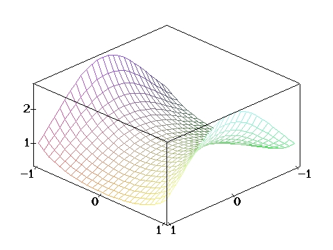
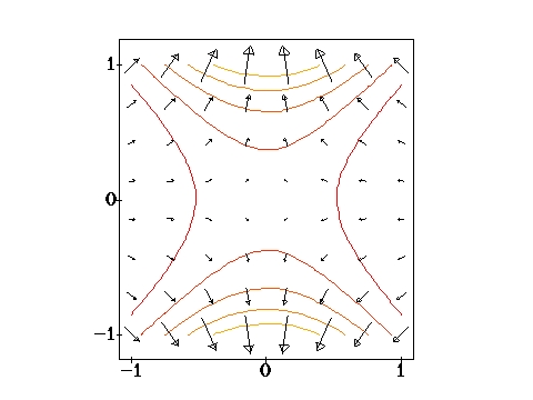
Here are the figures shown in class today. In each case, the first picture shows the (3-d!) graph of a function z = f(x,y), and the second shows the combined (2-d!) graph of the level curves and gradient of f.
(You might obtain better quality pictures using an external JPEG viewer rather than your browser.)

10/2/00

Here's the problem I mentioned in class:

Find the unit tangent vector T, the curvature K, and the principal unit normal vector N at the point (1,1) on the curve y=x³. The correct answers are: T = (i+3 j)/10^1/2 ; K = (3/5)/10^1/2 ; N = (-3 i+j)/10^1/2

Hints: A parameterization of the curve is r = t i+t³ j. Use the method at the end of Lesson 2 in the Study Guide.

9/27/00

For those of you without the 4th edition of the text, I have placed a copy of the homework problems for this week outside my office (please remove only to copy), and will try to have it put on reserve immediately. Starting next week, I will put copies of the homework on reserve each week until I can replace that with a copy of the text.

9/26/00

If you are using Maple to graph parametric curves, you can use the command "plot" for 2d curves, for example:

plot([cos(t),sin(t),t=0..2*Pi]);

but for 3d parametric curves you must use "spacecurve", for example:

with(plots):
spacecurve([t,t^2,t^3],t=0..1);

Note that the syntax of these 2 commands is different!

9/25/00

Pay careful attention to Examples 3, 4, 5, and 6 in §13.1.

Please note the corrected section numbers on the suggested problems for Lesson 2.

9/22/00

Make sure to read the note about the various editions of the text.

Make sure to read the grading policy.