|
|
|
We now show how these two techniques can be applied to find subalgebras of rank $l$ algebras, for $l \ge 4$. We begin by using slices and projections to find subalgebras of the exceptional Lie algebra $F_4$. We then show how to apply these techniques to algebras of higher rank.
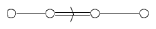
We apply the slice and projection techniques to the $52$-dimensional exceptional Lie algebra $F_4$, whose Dynkin diagram is shown in Figure 20. We number the nodes $1$ through $4$, from left to right, and use this numbering to label the simple roots $r^1, \cdots, r^4$. Thus, the magnitude of $r^1$ and $r^2$ is greater than the magnitude of $r^3$ and $r^4$. We color these simple roots magenta ($r^1$), red ($r^2$), blue ($r^3$), and green ($r^4$).
|
|
|
|
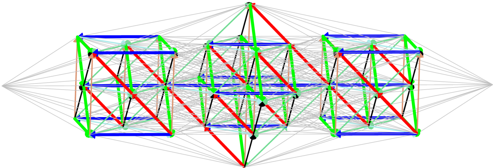
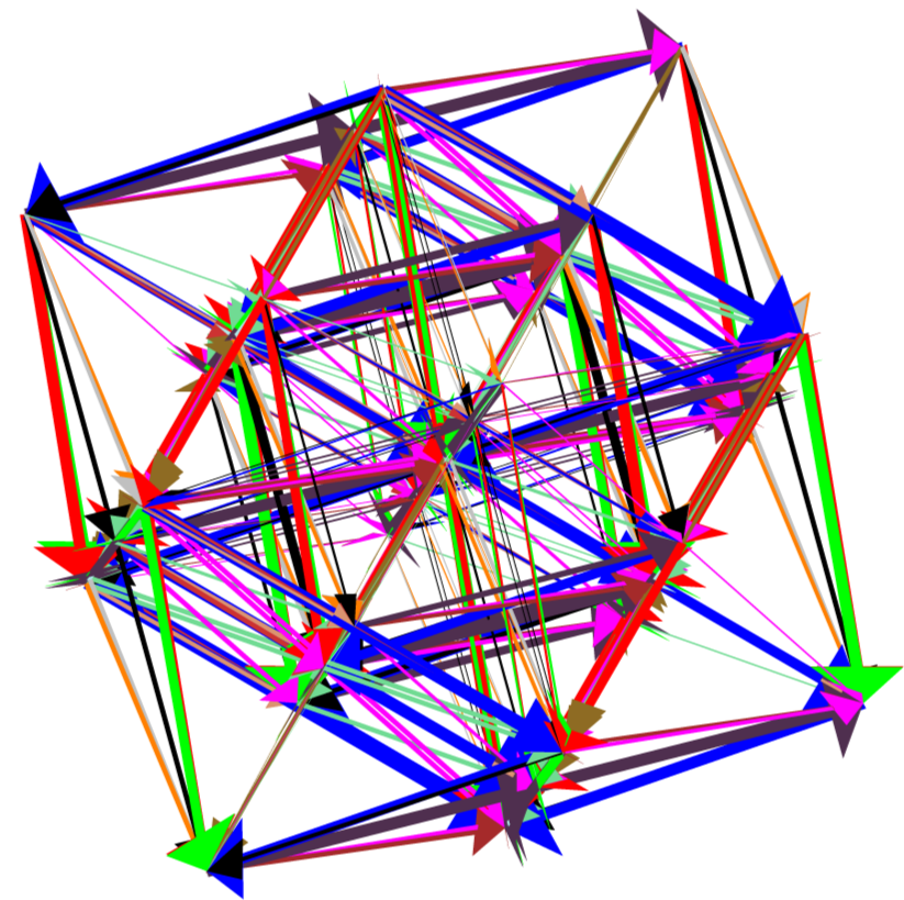
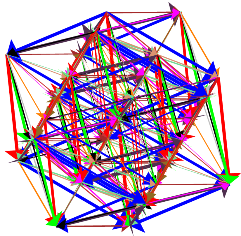
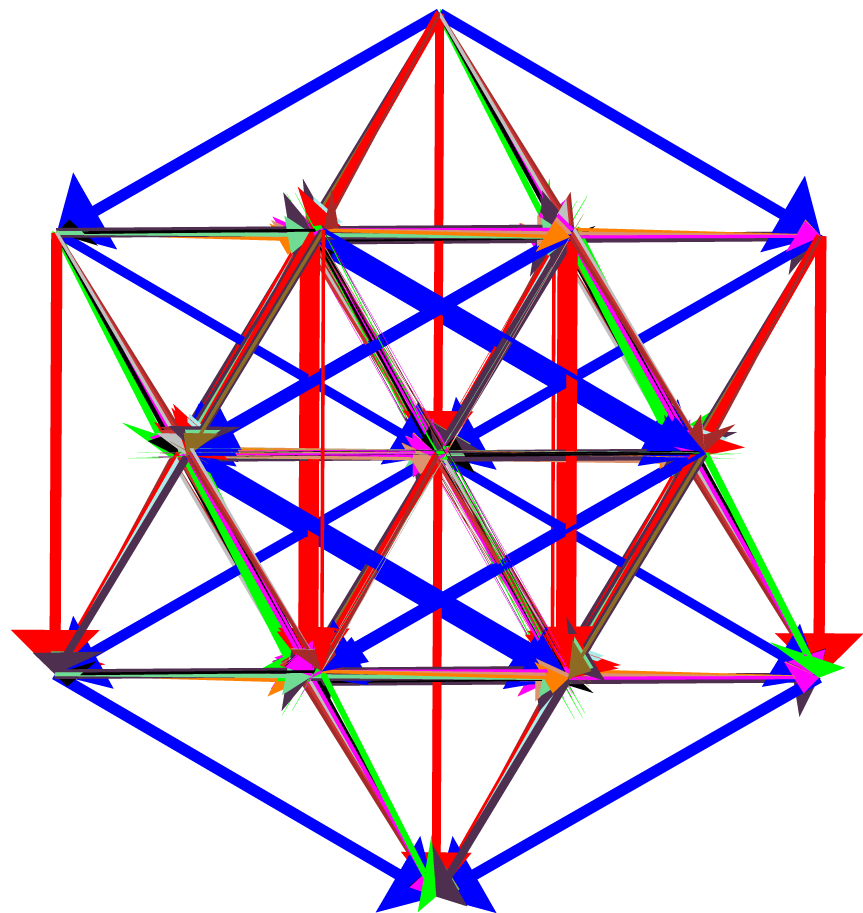
We consider the slicing of $F_4$ defined using roots $r^2$, $r^3$, and $r^4$. Laying the slices along the $x$ axis, the large number of grey struts in the resulting diagram, Figure 21, makes it difficult to observe the underlying structure of each slice, and so they are removed from the diagram in Figure 22. This diagram clearly contains three nontrivial rank $3$ root or weight diagrams. Comparing this diagram to the root diagrams in Figure 9, we identify the middle diagram, containing $18$ non-zero vertices, as the root diagram of $C_3=sp(2\cdot 3)$. The other two slices are identical non-minimal weight diagrams of $C_3$. Because there are $46$ non-zero vertices visible in Figure 22, it is clear that two single vertices are missing from this representation of the root diagram of $F_4$, which has dimension $52$.
|
|
|
|
|
|
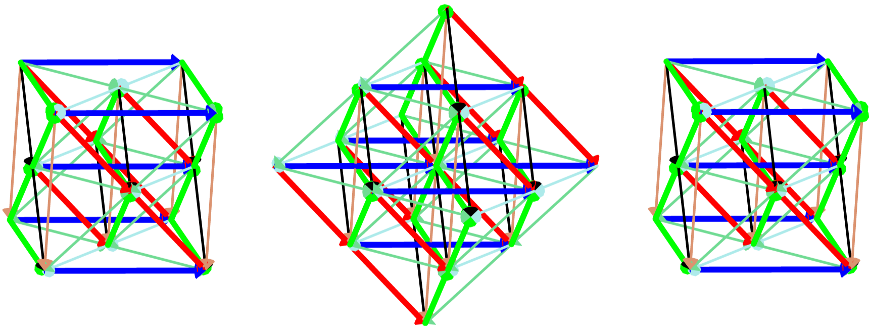
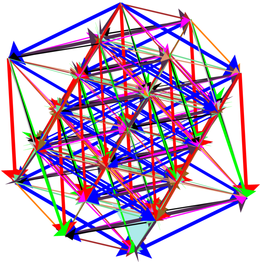
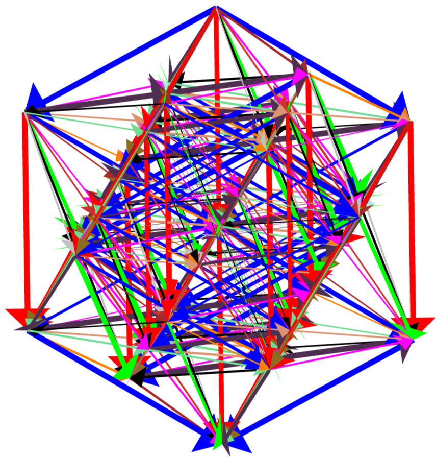
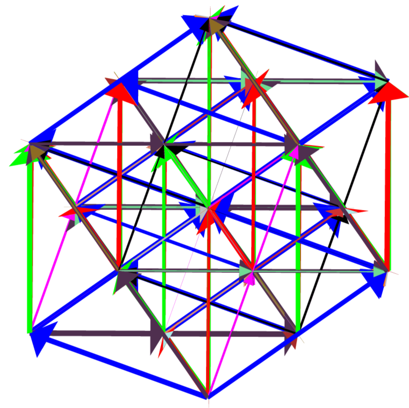
Figure 23 is the result of slicing the root diagram of $F_4$ using the simple roots $r^1$, $r^2$, and $r^3$. The center diagram again contains $18$ non-zero weights, which we identify as $B_3=so(7)$ using Figure 9. Hence, $B_3 \subset F_4$. Furthermore, as all $48$ non-zero vertices are present and there are $5$ nontrivial slices in the root diagram, we compare this sliced root diagram of $F_4$ with that of $B_4=so(9)$, which is shown in Figure 17, and see that $B_3 \subset B_4 \subset F_4$. An additional slicing of $B_4$ shows $D_4 =so(8) \subset B_4 \subset F_4$.
|
|
|
Given the $4$-dimensional root diagram of $F_4$, we can observe its $3$-dimensional shadow when projected along any one direction. However, as a single projection eliminates the information contained in one direction, it is not possible to understand the root diagram of $F_4$ using a single projection. We work around this problem by creating an animation of projections, in which the direction of the projection changes slightly from one frame to the next.
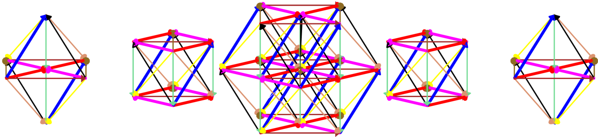
The Dynkin diagram of $F_4$ reduces to the Dynkin diagram of $C_3=sp(2\cdot 3)$ or $B_3=so(7)$ by eliminating either the first or fourth node. The simple roots $r^1$ and $r^4$ define a plane in $\mathbb{R}^4$, and we choose a projection vector $p_{\theta} = \cos \theta r^1 + \sin \theta r^4$ to vary discretely in steps of size $\frac{\pi}{18}$ from $\theta = 0$ to $\theta = \frac{\pi}{2}$ in this plane. Each value of $\theta$ produces a frame of the animation sequence using the projection procedures of section $3.2$. The resulting animation is displayed in Figure 24.
The result of each projection of $F_4$ is a diagram in three dimensions. We create the animation using Maple, and the software package Javaview is used to make a live, interactive applet of the animation. The Javaview applet allows the animation to be rotated in $\mathbb{R}^3$ as it plays. In particular, when $\theta = 0$, we can rotate the diagram to show a weight diagram of $C_3=sp(2\cdot 3)$, which our eyes project down to the root diagram of $B_2 = C_2$. Without rotating the diagram, the animation continuously changes the projected diagram as $\theta$ increases. When $\theta = \frac{\pi}{2}$, our eyes project the root diagram of $B_3 = so(7)$ down to the root diagram of $G_2$. However, it is also possible to rotate the animation to see the root diagram of $G_2$ at various other values of $\theta$. The interactive animation makes it easier to explore the structure of $F_4$.
This interactive animation can also illustrate an obvious fact about planes in $\mathbb{R}^4$. As $p_{\theta}$ is confined to a plane, there is a plane $P^{\perp}$ which is orthogonal to each of the projection directions. Thus, the projection does not affect $P^{\perp}$, and it is possible to see this plane in $\mathbb{R}^3$ by rotating the animation to the view shown in the sixth diagram in Figure 24. In this configuration, the roots and vertices in this diagram do not change as the animation varies from $\theta = 0$ to $\theta = \frac{\pi}{2}$. While this is obvious from the standpoint of Euclidean space, it is still surprising this plane can be seen in $\mathbb{R}^3$ even as the projected diagram is continually changing.
|
|
|
||
|
|
|
|
|
|
|
|
|
|
|
||
|
Here is the interactive animation in a separate window. |
||||
Of particular interest is the exceptional Lie algebra $E_6$, which preserves the the determinant of elements of the Cayley plane. As explained in Section $2.1$, this allows us to write $E_6 = sl(3,\mathbb{O})$. It therefore naturally contains the subalgebras $sl(2,\mathbb{O})$ and $su(2, \mathbb{O})$, which are identified as real forms of $D_5$ and $B_4$, respectively [13].
The projection technique can also be used to identify subalgebras of rank $E_6$. In one version, we project the root diagram of $E_6$ along one direction, thereby creating a diagram that possibly corresponds to a rank $5$ algebra $g$. We then apply the same pair of projections to our projected $E_6$ diagram and to the candidate root diagram of $g$. If these two projections preserve the number of vertices in the $5$-dimensional diagrams, it is possible to compare the resulting diagrams in $\mathbb{R}^3$. If we have identified the correct subalgebra of $E_6$, the resulting two diagrams should match for every pair of projections applied to the $5\textrm{-dimensional}$ diagrams.
Projections of rank $5$ and $6$ algebras can also be simulated using slicings of their root diagrams. This is done using the slice and collapse technique, which collapses all the slices onto one another in a particular direction. When using this technique, we draw the grey struts, as we are now interested in the root diagram's structure after the projection. This technique provides clearer pictures compared to the pure projection method.
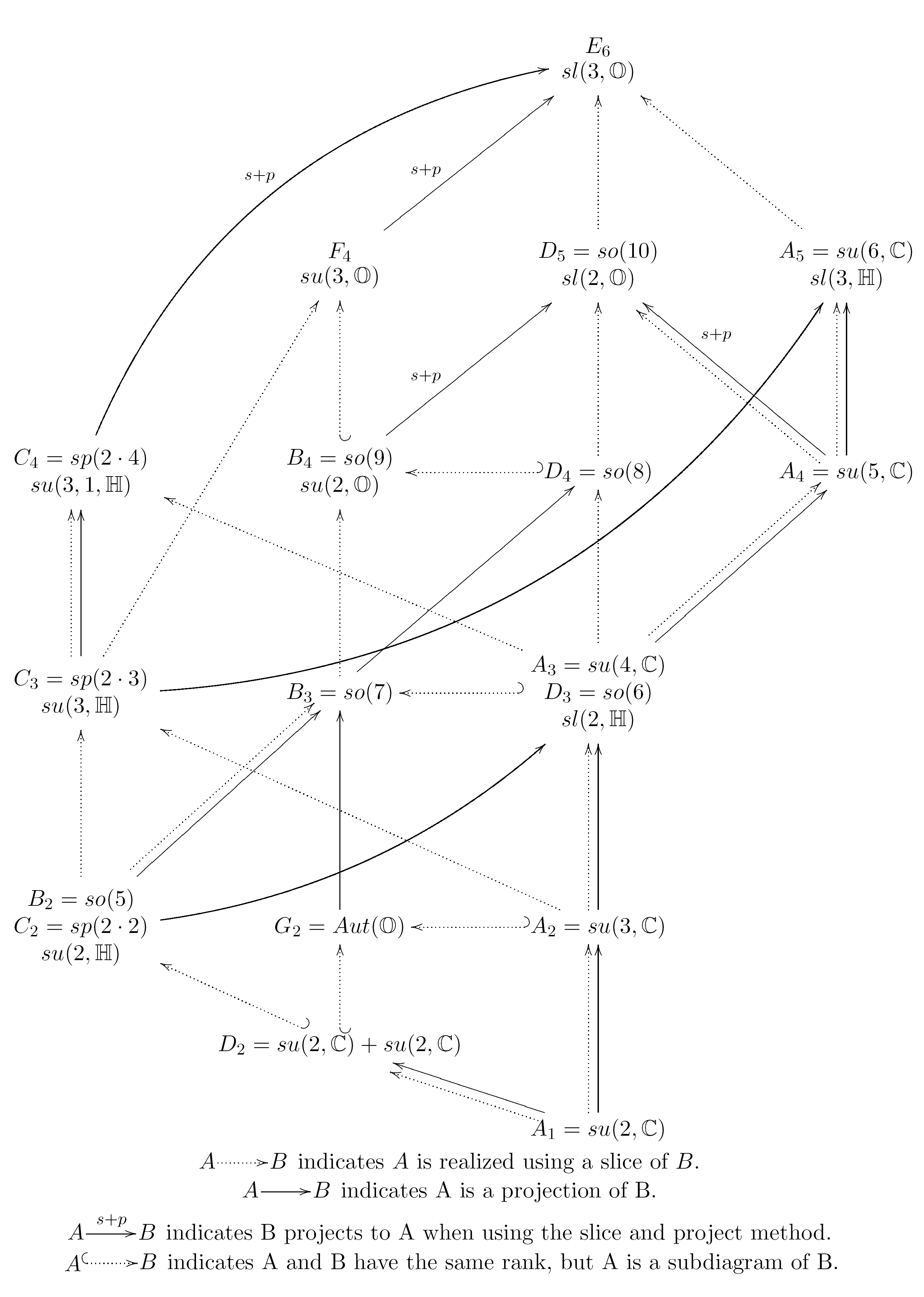
We list in Figure 25 the subalgebras of $E_6$ found using the slicing and projection techniques applied to an algebra's root diagram. As mentioned in Section $2.1$, we list certain real representations of the subalgebras of the $sl(3,\mathbb{O})$ representation of $E_6$ in the diagram. The particular real representations are listed below each algebra.
We use different notations to indicate the particular method that was used to
identify subalgebras. The notation  indicates
the slicing method was used to identify $A$ as a subalgebra of $B$. The
notation
indicates
the slicing method was used to identify $A$ as a subalgebra of $B$. The
notation  indicates that $A$ was identified as a
subalgebra of $B$ using the normal projection technique, while we indicate
projections done by the slice and collapse method
as
indicates that $A$ was identified as a
subalgebra of $B$ using the normal projection technique, while we indicate
projections done by the slice and collapse method
as  . If both dotted and solid arrows
are present, then $A$ can be found as a subalgebra of $B$ using both slicing
and projection methods. If $A$ and $B$ have the same rank, only the slicing
method allows us to identify the root diagram of $A$ as a subdiagram of $B$.
This case is indicated in the diagram using the notation
. If both dotted and solid arrows
are present, then $A$ can be found as a subalgebra of $B$ using both slicing
and projection methods. If $A$ and $B$ have the same rank, only the slicing
method allows us to identify the root diagram of $A$ as a subdiagram of $B$.
This case is indicated in the diagram using the notation  . Each of the
subalgebra inclusions below can be verified online [14].
. Each of the
subalgebra inclusions below can be verified online [14].
|
|
|
Lists of subalgebra inclusions are found in [12], which applies subalgebras to particle physics, and in [15], which recreates the subalgebra lists of [16]. However, the list in [15] mistakenly has $C_4$ and $B_3$ as subalgebras of $F_4$, instead of $C_3$ and $B_4$. Further, the list omits the inclusions $G_2 \subset B_3$, $C_4 \subset E_6$, $F_4 \subset E_6$, and $D_5 \subset E_6$. The correct inclusions of $C_3 \subset F_4$ and $B_4 \subset F_4$ are listed in Section $8$ of [16], but the $B_n$ and $C_n$ chains are mislabeled in the final table which was used by Gilmore in [15]. Although van der Waerden uses root systems do determine subalgebra inclusions, he mistakenly claims that $D_n \subset C_n$ as a subalgebra in Section $21$, which is not true since their root diagrams are based upon inequivalent highest weights.
In [9], Dynkin classified subalgebras depending upon the root structure. If the root system of a subalgebra can be a subset of the root system of the full algebra, the subalgebra is called a regular subalgebra. Otherwise, the subalgebra is special. A complete list of regular and special subalgebras are listed in [12]. All of the regular embeddings of an algebra in a subalgebra of $E_6$ can be found using the slicing method. In many cases, the projection technique also identifies these regular embeddings of subalgebras, but there are regular embeddings which can are not recognized as the result of projections. The special embeddings of an algebra in a subalgebra of $E_6$ can only be found using the projection technique.
Go to Conclusion