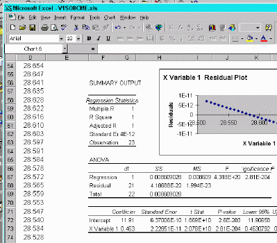
While Excel does a thorough job of providing statistical data from linear regression, the volume of data is overkill for our purposes:

Locating the relevant data can be confusing, and all the extraneous data clutters the worksheet. There is an easier way. We are interested in the slope, intercept and r2 values. Look at the sheet below to see how to do this:

Note the formula in the cell window:
=SLOPE(A20:A24,B20:B24)
This returns the slope value by designating the desired data
(SLOPE, INTERCEPT, RSQ)
followed by the range of y values (A20:A24), a comma, and the x values (B20:B24).
To do this, you have to have generated the slope and intercept. The best method is to reference the cells that hold these values. Then, generate a new series of y values, using slope, intercept and x values:
=+$H$36*B23+$H$37
references the slope as a constant value (hit function key F 4 ) in cell H36, the x value as a variable in cell B23, and the intercept as a constant value (F4) in cell H37. This formula may now be copied to every cell in a new column to generate calculated Y values. Now edit the plot to add the new series; you can turn off the marker to make it look nice.