Table of Contents
Typical Examples
We present here three examples that are fairly typical of junior-level coursework for physics majors, followed in each case by a brief discussion, emphasizing the challenges students have when applying their prior mathematical knowledge. Bear in mind that these examples arise shortly after students have learned the underlying mathematical concepts.
— TD & CAM, 3/15/14
The electric field above a line segment
Find the electric field a distance $z$ above the midpoint of a straight line segment of length $2L$ that carries a uniform line charge $\lambda$.
(David J. Griffiths, Introduction to Electrodynamics, 4th edition, Pearson, 2013, pages 64–65) 1)
Background
The electric field $\EE$ due to a point charge $q$ at the origin is \begin{equation} \EE = \frac{1}{4\pi\epsilon_0} \frac{q\,\rhat}{r^2} \end{equation} This leads through the superposition principle to the electric field of a linear charge distribution $\lambda$ along a curve $C$ being \begin{equation} \EE = \frac{1}{4\pi\epsilon_0} \int_C \frac{\lambda\,\widehat{\Delta r}\,d\ell'}{|\vec{\Delta r}|^2} \end{equation} where $\EE$ is regarded as a function of position $\rr$, and the integral is over the position $\rr'$ along the curve. Thus, $\lambda$ depends on $\rr'$, and $d\ell'=|d\rr'|$.
Solution
We have \begin{align} \rr=z\,\zhat \qquad \rrp&=x\,\xhat \qquad d\ell'=dx \nonumber\\ \vec{\Delta r}=\rr-\rrp=z\,\zhat-x\,\xhat &\qquad |\vec{\Delta r}|=\sqrt{z^2+x^2} \nonumber\\ \widehat{\Delta r}=\frac{\vec{\Delta r}}{|\vec{\Delta r}|} &= \frac{z\,\zhat-x\,\xhat}{\sqrt{z^2+x^2}} \end{align} Thus, \begin{align} \EE &= \frac{1}{4\pi\epsilon_0} \int_{-L}^L \frac{\lambda}{z^2+x^2} \frac{z\,\zhat-x\,\xhat}{\sqrt{z^2+x^2}}dx \nonumber\\ \EE &= \frac{\lambda}{4\pi\epsilon_0} \left[ z\,\zhat \int_{-L}^L \frac{1}{(z^2+x^2)^{3/2}}\,dx -\xhat \int_{-L}^L \frac{x}{(z^2+x^2)^{3/2}}\,dx \right] \nonumber\\ &= \frac{\lambda}{4\pi\epsilon_0} \left[ z\,\zhat \left( \frac{x}{z^2\sqrt{z^2+x^2}} \right) \Bigg|_{-L}^L -\xhat \left( -\frac{1}{\sqrt{z^2+x^2}} \right) \Bigg|_{-L}^L \right]\ \nonumber\\ &= \frac{1}{4\pi\epsilon_0} \frac{2\lambda L}{z\sqrt{z^2+L^2}}\zhat \end{align}
For points far from the line ($z\gg L$), \begin{equation} E \cong \frac{1}{4\pi\epsilon_0} \frac{2\lambda L}{z^2} \end{equation} This makes sense: From far away the line looks like a point charge $q=2\lambda L$. In the limit $L\mapsto\infty$, on the other hand, we obtain the field of an infinite straight wire: \begin{equation} E = \frac{1}{4\pi\epsilon_0} \frac{2\lambda}{z} \end{equation}
Discussion
- One major confusion here is the need to distinguish between $\rr$, which gives the functional dependence of the final answer, and $\rr'$, which gives the functional dependence of the integrand.
- Equivalently, students need to distinguish between the dummy variable $x$, which should not appear in the final answer, and the position $z$, which is a constant during integration, but the only variable in the final answer.
-
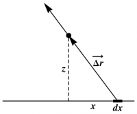 The problem statement in Griffiths includes a picture, showing $x$, $z$, a typical piece $dx$ of the line segment, and the vectors $\rrp$ and $\vec{\Delta r}$. This picture is crucial to the first step of identifying the components of $\rr$ and $\rrp$.
 - Notation such as $\EE=E\hat{E}$, in which base letters such as $E$ are reused for a vector ($\EE$), and the magnitude ($E$) and direction $\hat{E}$ of the vector, is common in physics, but rare in mathematics.
- The integrals themselves are doable, but not easy; ditto for the algebraic simplifications in the last step.
- The casual discussion of limiting cases at the end is an automatic reality check for physicists, but not yet second-nature for students. Furthermore, checking those limiting cases amounts to taking the leading term of a power series, a competency physicists expect students to have already mastered.
Solutions of Schrödinger's Equation
Find the general solution of the Schrödinger equation for a time-independent Hamiltonion.
(David H. McIntyre, Quantum Mechanics: A Paradigms Approach, Pearson Addison-Wesley, 2012, pages 68–70)
Background
The time evolution of a quantum system is determined by the Hamiltonion or total energy operator $H$ through the Schrödinger equation \begin{equation} i\hbar\frac{d}{dt}|\psi(t)\rangle = H|\psi(t)\rangle \end{equation} The energy eigenvalue equation is \begin{equation} H|E_n\rangle = E_n|E_n\rangle \end{equation} The eigenvectors of the Hamiltonion form a complete basis, so that \begin{equation} |\psi(t)\rangle = \sum_n c_n(t) |E_n\rangle \end{equation} We assume that $H$, and hence $|E_n\rangle$ and $E_n$, are independent of $t$.
Solution
Substitute the general state $\psi(t)$ above into the Schrödinger equation: \begin{equation} i\hbar\frac{d}{dt}\sum_n c_n(t)|E_n\rangle = H \sum_n c_n(t)|E_n\rangle \end{equation} and use the energy eigenvalue equation to obtain \begin{equation} i\hbar\sum_n\frac{dc_n(t)}{dt}|E_n\rangle = \sum_n c_n(t)E_n|E_n\rangle \end{equation} Each side of this equation is a sum over all the energy states of the system. To simplify this equation, we isolate single terms in these two sums by taking the inner product of the ket on each side with one particular ket $|E_k\rangle$. The orthonormality condition $\langle E_k|E_n\rangle=\delta_{kn}$ then collapses the sums: \begin{align} \langle E_k|i\hbar\sum_n\frac{dc_n(t)}{dt}|E_n\rangle &= \langle E_k|\sum_n c_n(t)E_n|E_n\rangle \\ i\hbar\sum_n\frac{dc_n(t)}{dt} \langle E_k|E_n\rangle &= \sum_n c_n(t)E_n\langle E_k|E_n\rangle \\ i\hbar\sum_n\frac{dc_n(t)}{dt} \delta_{kn} &= \sum_n c_n(t)E_n\delta_{kn} \\ i\hbar\frac{dc_k(t)}{dt} &= c_k(t)E_k \end{align} We are left with a single differential equation for each of the possible energy states of the system $k=1,2,3,…$. This first-order differential equation can be rewritten as \begin{equation} \frac{dc_k(t)}{dt} = -i\frac{E_k}{\hbar} c_k(t) \end{equation} whose solution is a complex exponential \begin{equation} c_k(t) = c_k(0) e^{-iE_k/\hbar} \end{equation} We have denoted the initial condition as $c_k(0)$, but we denote it simply as $c_k$ hereafter. Each coefficient in the energy basis expansion of the state obeys the same form of the time dependence, but with a different exponent due to the different energies. The time-dependent solution for the full state vector is summarized by saying that if the initial state of the system at time $t=0$ is \begin{equation} |\psi(0)\rangle = \sum_n c_n|E_n\rangle \end{equation} then the time evolution of this state under the time-independent Hamiltonian $H$ is \begin{equation} |\psi(t)\rangle = \sum_n c_ne^{-iE_n/\hbar}|E_n\rangle \end{equation}
Discussion
- This computation is very abstract! The state $|\psi\rangle$ could be a column vector, a function, or an element of some other vector space.
- The use of bra/ket notation for vectors is becoming standard in quantum mechanics, but forces students to translate their knowledge of linear algebra into a new notation.
- Note the reuse of labels when writing the eigenstate with eigenvalue $E_n$ as $|E_n\rangle$.
- The ability to pull operators through sums is “just” linearity, but not yet easy for students.
- The casual use of the Kronecker delta may be unfamiliar to students.
- An interesting feature of this presentation (and the book from which it comes) is the emphasis on using basis vectors to determine vector components. In the more familiar language of vector analysis, this is the statement that the $x$-component $F_x$ of a vector field $\FF$ is given by \begin{equation} F_x = \xhat\cdot\FF \end{equation} Thus, when determining the differential equation for $c_k(t)$, an explicit dot product is used, rather than simply equating the components of the vector. One could argue that this approach is unnecessary in this example, but it is crucial in situations where the given vector is not already expressed in terms of the desired basis.
Maxwell relations
Derive the Maxwell relation associated with internal energy.
(Ashley H. Carter, Classical and Statistical Thermodynamics, Prentice-Hall, 2001, page 134)
Background
For homogeneous systems, with a well-defined temperature $T$ and pressure $P$, the first law of thermodynamics becomes the fundamental thermodynamic relation \begin{equation} dU = T\,dS - P\,dV \end{equation} where $V$ is the volume of the system, $S$ its entropy, and $U$ denotes the internal energy.
Solution
The internal energy $U$ is a state variable whose differential is exact. Since the value of a mixed second partial derivative is independent of the order in which the differentiation is applied, we have \begin{equation} dU = T\,dS + (-P)\,dV = \left(\frac{\partial U}{\partial S}\right)_V dS + \left(\frac{\partial U}{\partial V}\right)_S dV \end{equation} The exactness of $dU$ immediately gives \begin{equation} \frac{\partial^2U}{\partial V\,\partial S} = \left(\frac{\partial T}{\partial V}\right)_S = \frac{\partial^2U}{\partial S\,\partial V} = -\left(\frac{\partial P}{\partial S}\right)_V \end{equation} The equality of the first derivatives, \begin{equation} \left(\frac{\partial T}{\partial V}\right)_S = -\left(\frac{\partial P}{\partial S}\right)_V \end{equation} is known as a Maxwell relation. Its utility lies in the fact that each of the partials is a state variable that can be integrated along any convenient reversible path to obtain differences in values of the fundamental state variables between given equilibrium states.
Discussion
- First of all, note the names of the variables: $T$, $S$, $P$, $V$, $U$; there's not an “$x$” in sight.
- It is not obvious which of these variables are dependent, and which are independent. A common feature of problems in thermodynamics is that equations express relationships between physical quantities, any of which can be regarded as independent in appropriate circumstances. The above exercise is typically followed by similar derivations starting from \begin{align} dH &= T\,dS + V\,dP \\ dA &= -S\,dT - P\,dV \\ dG &= -S\,dT + V\,dP \end{align} where $H$ is the enthalpy, $A$ the Helmholtz free energy, and $G$ the Gibbs free energy. Students find this changing role of the given quantities from one context to another to be quite confusing.
- This flexibility in the designation of independent variables leads naturally to the need to specify explicitly which quantities are being held fixed, as denoted above with subscripts. “The derivative of $V$ with respect to $P$” is ambiguous, since \begin{equation} \left(\frac{\partial V}{\partial P}\right)_S \ne \left(\frac{\partial V}{\partial P}\right)_T \end{equation}
- Manipulations such as these require comfort with differentials, yet differentials tend to be used in calculus only for linear approximations, a very different concept.
1)
With apologies to David Griffiths, we have used $\vec{\Delta r}$ in place of
“script-r vector”, which we have been unable to typeset.