• Maple is used to compute the full solution quantum mechanical solution to the hydrogen atom
• Students can visualize the probability density of the electron
• Students can connect various represent to the hydrogen orbitals they've seen in chemistry

Estimated Time: 20 minutes

Students use Maple to visualize the probability density distribution for the hydrogen atom orbitals with the option to vary the values of $n$, $l$, and $m$.

• Computers with Maple and the Maple Worksheet cfhydrogenvis.mw (Maple 13)

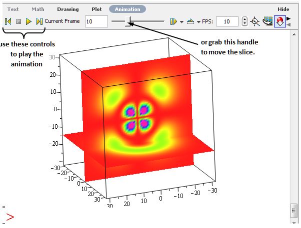
Before beginning this activity, it is helpful to discuss with students how one might plot a three dimensional scalar field like the probability density. After discussing some of their ideas, it is important to describe the method we use for plotting the probability density in three dimensions. We use color to represent the magnitude of the probability density. The Maple worksheet displays one static slice through the $x$-$z$ plane (with $y=0$) and a second cross sectional slice parallel to the $x$-$y$ plane. The plot is rendered as an animation so that one can vary the $z$-value of the slice parallel to the $x$-$y$ plane either by dragging the slider or playing the animation.

Note: This worksheet is very computationally intensive. On older machines and those with less RAM, it is sometimes possible to speed up the calculations by closing any unused plot windows and/or restarting each time you generate a new hydrogen orbital. If you still experience problems set the plottype to “static2” in the worksheet to get a static plot rather than an animation

You may find the following worksheets useful for in class demonstration.

The Maple worksheet cfhydrogenvis_demo.mw is a simple worksheet that you can use to easily display single or linear combinations of hydrogen wavefunctions. This worksheet also makes it possible to look at linear combinations as a function of time.

The Maple worksheet cfhydrogenvis_array.mw displays an array of static plots of several hydrogen atom orbitals. This worksheet can be used as a tool for guiding the discussion that flows from this activity.

Students will often ask why the plots in this worksheet are different from the plots most commonly found in text books. We try to help them see that the plots most commonly included in text books are iso-probability plots. We explain that the iso-probability plots are surfaces of uniform probability. To see this in the maple worksheet, imagine looking at only shows one color.

Some good questions that help students focus their exploration include:

• What do you notice about the shape of the probability densities when $l=0$?
• Do you notice any symmetries in the orbitals?
• How do the orbitals vary with $n$, $l$, and $m$?
• Since all the orbitals are axially symmetric how do you think one might represent non-axially symmetric electron wavefunctions like the the chemistry orbitals $p_x$, $p_y$, etc. using these orbitals?

Note: Depending on the speed of the computer used and the complexity of the wave function, Maple can take up to a few minutes to calculate the probability distribution animation. We recommend you test out the worksheet on the computers you plan to use so that you can plan accordingly.

We often wrap up this activity by trying to tie their observations of the shapes of the orbitals back to what they know about hydrogen orbitals from chemistry and modern physics.

Some questions we use to guide the wrap-up discussion include:

1. What do the orbitals look like when $l$ is zero?
2. What do you expect/observe for high values of $n$ with $l=0$?
3. Choose $n$ equal to some larger value ($n=6$) and $l$ equal to the largest value possible, ($l=5$). Now compare the shapes of the orbitals for $m$ a maximum ($m=5$) and $m=0$. Think about these orbitals from the perspective of moment of inertia in the classical sense. Do the shapes of the orbitals you observe make sense with regard to the associated eigenvalues for the $z$-component of the angular momentum? Explain what about the shape of the orbitals makes sense? Make a prediction about how the shape of the orbitals will change as you vary the value of $m$ from its maximum value to its minimum value.