11/18/06 (CP/JDI)
General Introduction on How to Use of a Spreadsheet1. There are PC's available for use during the laboratory in rooms 311 and 313. Turn the power on for the computer and monitor. Usually these are all powered up from a nearby power strip. The printer may operate from its own power strip or be on the network - so generally there is no need to turn this on and off.
2. There are two common spreadsheet programs: Excel and QuattroPro. The following directions are specific for Excel, but all spreadsheets operate about the same way. Use the mouse and Left Click (L-Click) on the Excel icon on the bottom tool bar; or double L-click on the Excel icon on the desktop shell. The left mouse button is used to point and click on a menu item to select that item. Clicking the right mouse button activates a secondary menu pertaining to the item you are pointing to.
3. A blank spreadsheet (below called Book2) will appear with a menu bar at the top of the screen. The columns are labeled with letters of the alphabet; the rows are numbered down the left side. Each position described by a column/row is called a cell. Move around the spreadsheet and select different cells by either using the mouse, the arrow keys or the PageUp/PageDown keys. The line above the work area, but below the menu bar shows the highlighted cell address (e.g., A1) and the contents of the cell are shown after the = sign (this is empty below). This is the space that is used to type in equations and commands.
4. The mouse is used to point and select. For example, point to
an option on the top menu bar and select it by L-clicking - a drop down menu will appear.
Another way to find options is to right clicking the mouse
(or R-Click) on any cell or block - this will bring up a
secondary menu for the cell properties. From this secondary menu you can edit or customize
properties for the cell.
5. THERE ARE TWO VERY USEFUL THINGS TO KNOW:
The Help Screen can be called up at any time by pressing the <F1> key (this is the universal access to Help) or clicking on Help on the tool bar of any menu.
AND
To undo something, use the <Esc> key to go back,
step by step, or use the mouse to point and click on the outside of any open menu box,
chose Cancel, or go to the top menu bar and select Edit-Undo.
6. Explore around the top menu bar and see what operations are available. Go to Help on the top menu and look up how to enter a formula to calculate a value. First try the MicroSoft Excel Help (this is assisted.) Next use Contents and Index. If you use the Contents and Index, start by typing "formulas" this will bring up all the help on this topic. From the list, L-click "entering" and select the Display button at the bottom of this prompt
7. Saving and Managing files. Always save your work in a file and get into the habit of re-saving frequently! It is better to be safe than sorry! To save a file, go to the top menu bar and select File - Save As. At the top of this prompt box, Save in should point to the drive in which you have a diskette, usually this is the A: drive. In GBAD 311 you may save files temporarily to the D: drive or in your own folder on the server (Bitbucket.) All local files may be erased at any time by The Management, so the C and D drives are not secure! Get in the habit of carrying a 3.5 inch diskette. After you have set up the file, you can use File-Save to update the file without changing the output file address and type.
Enter a filename at the bottom of the prompt box. The File name is your choice. The filename will automatically be fitted with an extension, .XLS is used by Exce. Note: most software is not backwards compatible. If you want to convert your file to another format to be used with other software, check to see what Save as type's are available. You must take care to save your file in a compatible format. Don't expect to open an Excel 2000 spreadsheet with an older version of Excel; instead, plan to save the file in the older file type version.
Always close the file that you are working on before removing the diskette from the drive. Select File - Close, or select X in top right most corner of document window. Many a student has been unhappy to find that the file they just spent an hour working on can not be re-opened because they removed the diskette before closing the file!
8. When you are finished working, exit the software by selecting from the top menu, File - Exit or select the X in the upper right corner of the open screen. Finish by shutting down the system at the end of the day. To do this go to the Start button on the bottom tool bar and, select Shut Down. If you are in room 311, select Log on as Another User. If you are in room 313, Shut Down the computer and turn off the system at the power strip.
9. Setup some data to practice with. Enter the following numbers in columns A and B:
Next fill in column A to cell 10 by highlighting cells A1 through A10
(do this by L-clicking and dragging down the column.) Now select from
the top menu bar Edit - Fill - Series to
generate a set of numbers in the highlighted area of the spreadsheet. The Fill
command prompts you to enter:
Series in -this is where you want the values to be
added - either a column or row
Type - in this example, select Linear.
Step value-this is the increment that will be added to
the first value to make the second entry, and all the successive values in the highlighted
area.
Stop value- this is the last value in the area. This
can be left blank since you have already defined the area to fill in.
Repeat the fill column procedure for Column B. Your spreadsheet should now look like:
Go to the third column, cell C1, and enter a formula that will multiply the value in A1 by 10.
To do this, type in the following formula: = A1*10 then press Enter. The function is evaluated and the value will appear in cell C1. (When the cell is highlighted (selected) the formula appears on the formula line.)
Now you will use one of the MOST IMPORTANT operations in spreadsheets ! There is a very easy way to apply this calculation down the entire C column, or anywhere else you like for that matter. This is simply done by using the Copy and Paste commands. Copy means that the contents of the highlighted cell (here cell C1) will be saved into the computer clipboard memory upon executing the Copy command, and then that information can be subsequently Pasted into another part of the spreadsheet (here C2 through C10). There are at least 3 ways to get to the editing functions. For example, you can get to Copy:
(1) from top menu, select Edit - Copy
(2) highlight cell of interest and simultaneously press the copy hot-keys <Ctrl> C
(3) or R-click the mouse on the selected region and select Copy.
After you have copied the formula in C1 into the clipboard, you will Paste it into C2 through C10. Highlight C2 through C10 and then do one of the following:
(1) select Edit-Paste from the top menu
(2) press the paste hotkeys, <Ctrl>V
(3) or R-Click and select Paste.
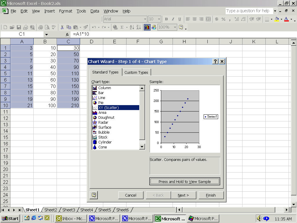
10. Graphing. In Excel, a graph is called a Chart. Select Insert - Chart and you will be guided through 5 steps to build a graph. A normal XY graph is called a Scatter Chart so select Type as Scatter.
Entering axes and editing graph:
There are several ways to enter the X and Y columns into the Chart. One is to first highlight the X and Y columns, then go to Insert-Chart.
If the Chart is already a part of your spreadsheet, select the Chart border, then press the right mouse button to call up a menu go to Source Data. Enter the columns containing the X and Y data by L-clicking in the spreadsheet directly and then highlighting the column, press enter or select the sheet icon to return to the chart building menu. Repeat for the Y column.
After the graph is built it can be sized, moved and edited. For example, to edit a region of the chart, L-Click to select the region (blinking cursors will show what has been selected), then right click to call up the specific menu. For example, L-Click to select the X axis, then R-Click, and go to Format axis which has multiple options that can be edited.
Multiple sets of data for one set of X data can be added by selecting Source Data.
Step 1: Select X and Y data points, open Chart wizard. Select XY(Scatter) and press and hold bar to preview graph. See if it looks right. :
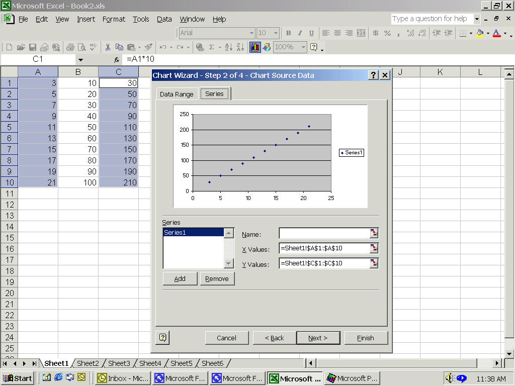
Step 2: Select the Series tab at the next screen. If the X and Y axes need adjusting, do it here. You can also add additional yseries if you want.
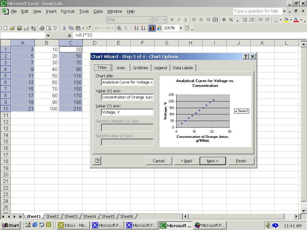
Step 3. Add titles and units to the graph and both axes.
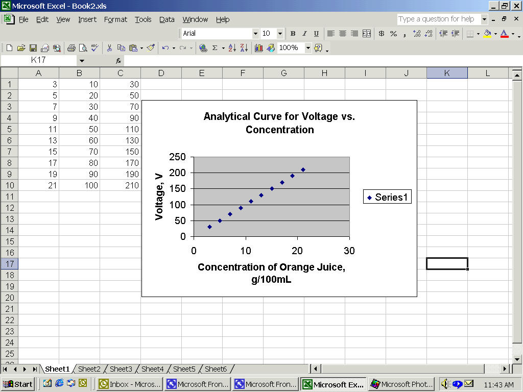
Step 4. Locate the graph in the spreadsheet for easy viewing with data.
R-clicking on a cell or component of a graph or table calls up a secondary
menu to select from, e.g., display a graph and R-click on the x-axis to edit attributes,
units, scale, tic marks, etc.
Many times it is helpful to use Markers, or symbols,
on the Y axis to show the actual data points on your graph. On the other hand, if a
curve is fitted by using linear regression, for example, this is displayed on the graph as
as a line only, with no markers. Select the entire line and right click, from there select
Format data series. Select a Line and Marker type, and check out the other properties that can be set.
See Chart Options to edit the titles for graph and
axes, text fonts, legend, gridlines, etc. (Note: the symbol font can be used
to input Greek symbols).
To get a hardcopy of the chart only, select the chart (i.e., designated by a highlighted chart border), then select File- Print. Alternatively, to print the spreadsheet text and inserted graph, block out the entire area then File- Print. Look under Page-Setup to select landscape format (11" across, 8 1/2"down) instead of the standard portrait format. In Excel there is also an interactive Page Break View that is useful for setting page breaks for long spreadsheets.
Simple least squares analysis, or linear regression, for fitting data to a model.
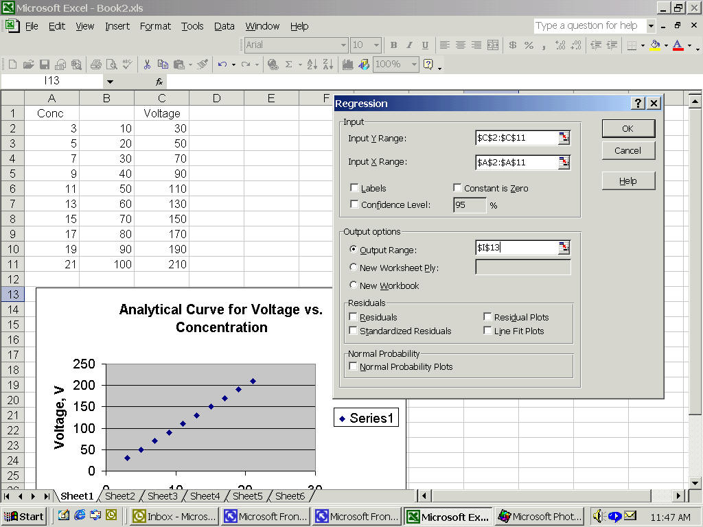
11.Select Tools-Data Analysis-Regression. If you don't find Data Analysis on the menu you must Add-In the function for Excel (go to Tools - Add Ins, and from there select Analysis ToolPak)
Set the Input Range (select X and Y points to be used in analysis) and set the Output Range (this is a space in the spreadsheet where the output of the calculation will be placed).
If you want the y-intercept to be zero, select Constant is Zero, otherwise the y-intercept will be calculated.
Output option can be set to either a section of the current page (Output Range) or set to a new sheet in your file called a Worksheet page (New Worksheet Ply) (notice the labelled tabs at the very bottom of the spreadhsheet-called Sheet1, Sheet2, etc, each one is a separate workspace).
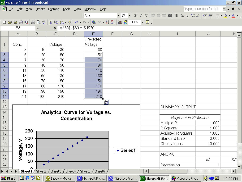
For this fake data, the fit is TOO good, but the results of the linear regression are given in a table. We are most interested in R Square, Intercept and Slope.
| SUMMARY OUTPUT | ||||
| Regression Statistics | ||||
| Multiple R | 1.000 | |||
| R Square | 1.000 | |||
| Adjusted R Square | 1.000 | |||
| Standard Error | 0.000 | |||
| Observations | 10.000 | |||
| ANOVA | ||||
| df | SS | MS | F | |
| Regression | 1 | 33000 | 33000 | #NUM! |
| Residual | 8 | 0 | 0 | |
| Total | 9 | 33000 | ||
| Coefficients | Standard Error | t Stat | P-value | |
| Intercept | 0.00 | 0 | 65535 | #NUM! |
| X Variable 1 | 10.00 | 0 | 65535 | #NUM! |
A useful function in the Residuals section is Line Fit Plots-this generates a chart with both the actual Y data and calculated predicted Y against X.
L-Click on the data points and then R-Click to call up the options menu. At this point, add a Trendline which will add an additional data series to the graph automatically from a predicted model for a set of Y data. Several model types for the trendline are available to choose from: linear, polynomial, exponential, etc. It is also useful to include the fitting equation and coefficients directly on the graph-do this by selecting Options in Trendline and checking boxes at the bottom of the prompt.
Alternatively, once you have the slope and intercept values from the linear regression analysis, you can calculate a predicted Yset and plot it as a second series yourself. Sometimes it is useful to get a list of the Residuals and Residual Plots. This can be helpful if you are trying to select between fitting models. Residuals are the difference between the actual Y-values and the calculated Y-values based on some assumed model (e.g., linear, polynomial, exponential, etc.)
Select OK when done to perform the regression.
Move the cursor over to the Regression Output block to view the regression parameters (note: the output may be on another sheet in your file-see above).
The automatic chart showing the comparison of calculated versus measured Y's is to the right of the output block. More information is returned than is normally useful. The important parameters are:
Slope (or X Variable 1)
Intercept
Standard Error
Adjusted R
It is often useful to consider the R Square value since this shows the correlation of the data with the model.
There are several other ways to get the fitting parameters and associated errors. Look in th MS Excel Help Topics for definitions of terms and equations used for:
LINEST (line statistics) and
Statistical Functions in the linear regression analysis tool.
ANOVA is "analysis of
variance".
Note that the Standard Error (or function STEYX) is defined
as the standard error of the predicted y-value for each x in the regression. The standard
error is a measure of the amount of error in the prediction of y for an individual
x.
An y-expectation value can be predicted using the FORCAST function.
NOTE: The Standard Error in the slope is the same as the standard deviation in the slope, however, for most spreadsheet programs, the Standard Error in the intercept is not the same as the standard deviation for the intercept. Therefore, it is strongly recommended that you use the following procedure to obtain the standard deviation in the Y- intercept for purposes of propagation of errors treatment. The following "trick" is not in the spreadsheet manuals.
12. After fitting your data, you now have the parameters a and b in the equation for a first order polynomial:
Y = a X0 + b X1
or in this simple case, a straight line:
Y = (intercept)1 + (slope)X
a. Program the spreadsheet to calculate a set of Y values for the observed set of X values using the slope and intercept just determined:
i. Enter the label "Predicted Voltage" in cell E1.
ii. Enter the formula for a straight line in cell E2 and use the cell address of the slope (J30) and the cell address of the intercept (J29) not the actual numbers (look in the Regression Output block to confirm the addresses). (Note: The $ before the column/row make these addresses absolute, so that they are not updated as you use the copy command. Highlight cell E2, point and click on the cell containing the slope, it is now automatically entered into your equation, now, press <F4> to make the cell absolute, continue entering the rest of the formula.)
iii. Once the formula is entered in the cell
E2, copy the formula down the
E column.
This is a good time to save the spreadsheet file!
iv. Add this new 2nd Series to your existing graph as the calculated Y values, column E. Click on the graph and look for Source Data-Series-Add.
13. Fitting of Non-Linear Data
If your X-Y data do not possess a linear relationship, you can use multiple least-squares analysis. To attempt to fit your data to a higher order polynomial or other function. For example,
Y = aXo + bX1 + cX2...
When you use the Linear Regression function, select the Independent Variable to include all X columns. Also set the Y-Intercept to Zero not Compute.
In the Regression Output block, you will see multiple columns for the values of a, b, and c, etc., coefficients, and the standard error for a, b, and c, etc., coefficients.
Note that this procedure can be extended to higher order polynomials or other functions of X (e.g., eX) by adding the appropriate column.
It is informative to generate a curve using the fitted coefficients for the various orders of X and display this on the graph as a line and use Markers only for the data. Producing a smooth curve for the generated line from a polynomial requires a little more effort than it does for a straight line. You need to generate points that are more closely spaced and have a larger range than the actual data does. To do this, start by leaving a blank row below your Y and X data values. Starting in the X axis column, fill in 20 or so values that will encompass the actual X data values. Using the coefficients reported in the Regression Table, generate the Ycalc values for these new X values, as well as the actual X data values. For the Graph Axes, set the entire X column, including blank row, and for the Y axis, set the entire Y column, including the blank row.
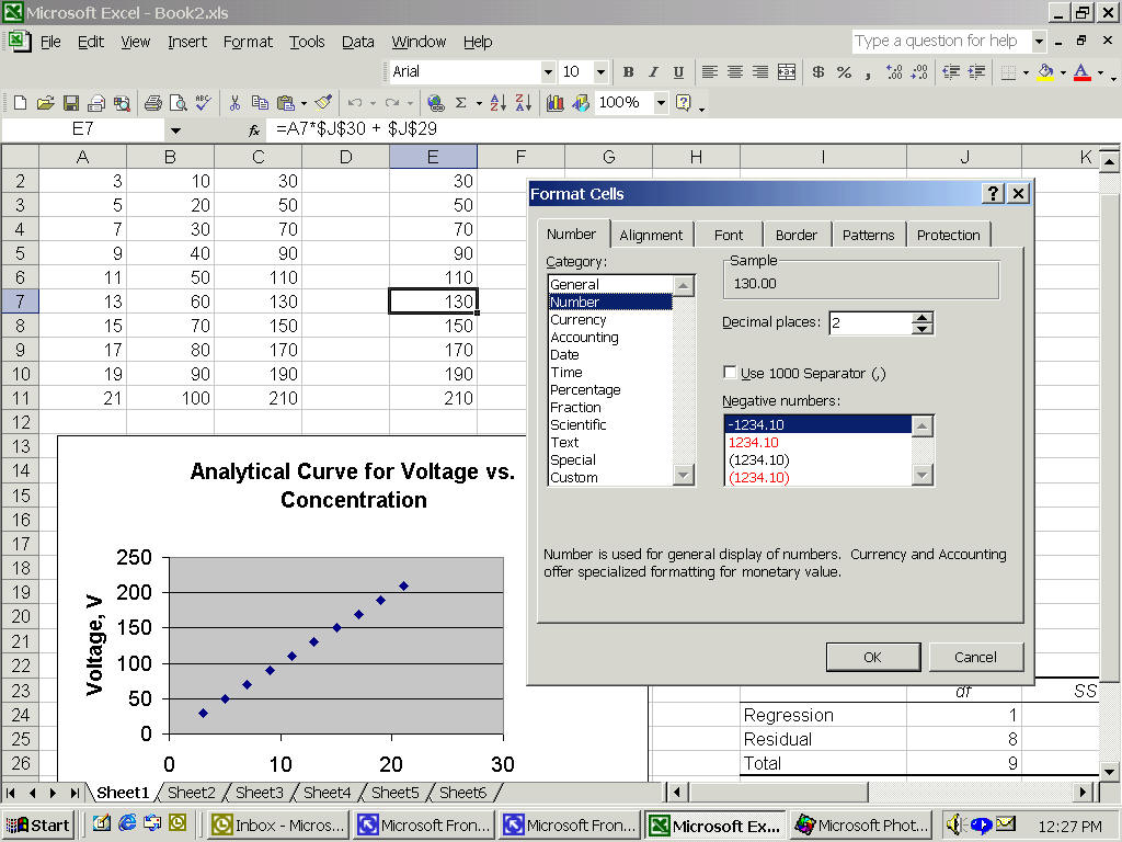
14. To adjust the display format for a block of the spreadsheet, point to a cell, or select a block, and press the right mouse button for Cell Properties:
16. Text printing.
If you are in GBAD 313, you can select the HP1220 color printer from File - Select Printer for color print jobs only. Do not send black and white printing to this queue.
Select the block of spreadsheet that you want to print. Select File - Print Preview to see how the final copy will look on screen before printing to paper. Look in Print Setup to change from portrait to landscape, set the margins, etc., before actually sending the job to the printer. In Excel there is also an interactive Page Break View that is useful for setting page breaks.
17. Importing data from an ASCII data file: Position the cursor in a cell where you want the data to be inputted into the spreadsheet, and select: Data -Text to Column. You will be directed to edit how you want the data inputted.
Put your floppy diskette in drive A and select A:\ *.* to see what files are on your diskette. Highlight the file you want to bring into the spreadsheet, and select OK.
A REAL APPLICATION.
Suppose you have experimental data that illustrates the temperature dependence of the equilibrium constant (Keq) for the isomerization of cis to trans 2-butene. You are curious whether this reaction is feasible or not, so you want to determine the reaction enthalpy and entropy, and to know whether these are significant.
Overview
The first step is to enter the temperatures and the corresponding Keq values (i.e., the data). Next, enter the necessary equations, and calculate the absolute temperature, lnKeq, 1/T, and
DG0.1. Start by labeling the columns. Position the cursor in the A1 cell, type the following labels, one by one, pressing the right arrow key (-
<) after each entry:
Cell [A1] [B1] [C1] [D1] [E1] [F1]
Label Temp,o-C K-eq o-K lnK-eq '1/T del-G
Note on [E1]: Use a tic mark ('), the caret (^), or the quotes (") to signify that a number is being used as a label (i.e., alpha-numeric), not in a calculation. Each of these marks also controls the alignment of the label in the cell ('=left, ^=center, "=right). I
2. Fill a Block with some test data (as described earlier). Set A2..A6 as the Block, and use 60 as the Start value, 20 as the Step value. Use the same method to fill in column B, Keq, with numbers from 7 to 3. Now enter the formulas used to calculate the other quantities.
If you make a mistake and wish to edit the contents of a cell, highlight the cell, and point to the dialogue box near the top of the screen that shows the contents of the cell, and click on the open dialogue box .
a. Highlight cell C2.
Type: =A2+273.15
Result: The Celsius temperature in cell A2 will be converted to Kelvin and this value (333.15) will be located in cell C2. Note: a formula starting with a cell address (e.g. A2) is preceded by a "=" so that the equation editor recognizes what follows as a value, not as a label.
b. Position the cursor in D2.
Type: =@ln(B2)
Result: This will use one of the pre-programmed functions, "ln", to calculate the natural log of the value in cell B2. The value for lnKeq (1.94591) will be located in cell D2.
c. Position the cursor in E2:
Type: =1/C2
Result: This will find the reciprocal of the Kelvin temperature (0.003002), and store the result in cell E2.
d. Position the cursor in F2:
Type: =-1.986*C2*D2
Result: This will calculate RTlnKeq (-1287.48) and store it in cell F2.
4. One of the great benefits to using a spreadsheet for data analysis is that a formula set up in one cell, can be used to extend the calculation on to other similar cells. The Copy command is used to do this. (See point 8 above).
Once you have the spreadsheet set up, Save it! Your spreadsheet should look something like the following table:
| Temp, oC |
K-eq |
oK |
lnK-eq |
1/T |
del-G |
60 |
7 |
333.15 |
1.9459 |
0.003002 |
-1287.48 |
80 |
6 |
353.15 |
1.7918 |
0.002832 |
-1256.66 |
100 |
5 |
373.15 |
1.6094 |
0.002680 |
-1192.72 |
120 |
4 |
393.15 |
1.3863 |
0.002544 |
-1082.41 |
140 |
3 |
413.15 |
1.0986 |
0.002420 |
-901.429 |
(Note: The table was pasted into this WordPerfect document by first using the Copy command under Edit in QPW, then the Paste command under Edit in WordPerfect. Any highlighted block can be stored temporarily in the Windows Clipboard while the operator changes from one Windows application to another. )